Ultrasound and NDT (coming from k-Wave)
Deepwave is used for medical ultrasound, photoacoustics, and non-destructive testing (NDT) as well as for seismic imaging. The wave physics is the same; what differs is the length and time scale (millimetres and microseconds rather than metres and seconds), the excitation (tone bursts rather than Ricker wavelets), and the acquisition (extended transducer elements rather than point sources). This page collects the Deepwave features and conventions that matter for these applications, and maps them onto the vocabulary of k-Wave, the established ultrasound simulation package, for readers arriving from there. For a broader tool comparison see Choosing a wave-propagation package.
Every code block below is an excerpt from one script, docs/example_ultrasound.py, which runs end to end and checks its own answers. It is written in a single unit system (millimetres, microseconds and megahertz) from the first line to the last, and it is run in Deepwave’s continuous integration, so this page cannot drift away from something that works.
Concept mapping from k-Wave
k-Wave | Deepwave |
|---|---|
| the model tensor’s shape, |
| the propagator model tensors: |
| constant-Q, single-mechanism SLS attenuation via |
| the initial wavefields |
|
|
|
|
|
|
| |
built-in time-reversal reconstruction | gradient-descent reconstruction through the differentiable propagator (Photoacoustic initial-pressure reconstruction) |
Choosing units for ultrasound
Deepwave itself is unit-agnostic: it only ever combines your numbers in dimensionless groups (the Courant number \(c\,\Delta t/\Delta x\), and the product of frequency and time step). You may therefore work in any single consistent system of units – the results are identical – provided every quantity uses it. The one requirement is consistency: grid_spacing, dt, the wave speed, and pml_freq must all refer to the same length and time units.
For ultrasound scales the cleanest choice is millimetres, microseconds, and megahertz, because it makes the numbers order-unity:
Quantity | Unit | Example value |
|---|---|---|
length / | mm |
|
time / | µs |
|
speed ( | mm/µs |
|
frequency / | MHz |
|
In this system a 3 MHz tone burst in water resolves a 0.5 mm wavelength, and the Courant number on 0.1 mm cells with a 0.01 µs time step is \(1.5\times0.01/0.1 = 0.15\). The equivalent SI setup (metres, seconds, m/s, hertz) – dx = 1e-4, dt = 1e-8, v = 1500, pml_freq = 3e6 – is exactly as valid and is what the worked Photoacoustic initial-pressure reconstruction uses; pick whichever keeps your numbers readable.
The example script opens by fixing that system once. It uses 0.05 mm cells rather than the table’s 0.1 mm, buying ten cells per wavelength instead of five, which is what Deepwave’s own resolution check asks for:
"""Focused ultrasound: a delay-focused array and a fluid-solid interface.

Everything here is in one unit system: millimetres, microseconds and
megahertz. Nothing converts between unit systems, because there is nothing
to convert -- Deepwave only ever combines these numbers in dimensionless
groups.

Part 1 builds the two excitation wavelets ultrasound and NDT use. Part 2
drives a linear array element with a focusing delay law and measures where
the beam really focuses. Part 3 puts water over bone and measures the
fluid-solid reflection coefficient.
"""

import math
import os

import matplotlib.pyplot as plt
import torch

import deepwave
from deepwave import elastic, scalar, transducers
from deepwave.wavelets import gaussian_pulse, tone_burst

# ``DEEPWAVE_SMOKE=1`` shrinks this example so that it can be run quickly
# as an automated check; the default sizes are the ones the text describes.
smoke = os.environ.get("DEEPWAVE_SMOKE") == "1"

# --- section: units ---
# One unit system throughout: mm, microseconds, MHz.
dx = 0.05  # mm cells (50 um): 10 cells per wavelength at 3 MHz in water
dt = 0.01  # microseconds (10 ns)
v_water = 1.5  # mm/us, i.e. 1500 m/s
rho_water = 1.0  # water density, in whatever mass unit you like
freq = 3.0  # MHz: the transducer's centre frequency

wavelength = v_water / freq  # 0.5 mm
cells_per_wavelength = wavelength / dx  # 10
courant = v_water * dt / dx  # 0.3
print(f"{cells_per_wavelength:.1f} cells/wavelength, Courant {courant:.2f}")

# `transducers` works in grid cells, so the speed it wants is a speed in
# cells per unit time. That division is the only conversion in this script.
c_cells = v_water / dx  # 30 cells/us
That last division is the only unit conversion in the script. deepwave.transducers measures positions in grid cells, so the speed it needs is a speed in cells per unit time; divide your physical speed by your cell size and the delays it returns come back in the time unit that matches your dt. Nothing in the module needs a grid_spacing of its own.
Note
You no longer have to set pml_freq by hand at ultrasound scales. When it is not given, Deepwave infers it from the peak of your source amplitudes’ spectrum, in your own frequency unit – so a 3 MHz tone burst gives 3.0 in the MHz system above, or 3e6 in SI. Deepwave 0.0.27 and earlier instead used a fixed 25, a seismic dominant frequency, which at ultrasound scales is effectively zero: it detuned the PML, let the model edges reflect, and made the grid-cells-per-wavelength check compare against a kilometre-scale wavelength, so it never fired. Wherever the inferred value is anything other than exactly 25, Deepwave warns once to point out that the numbers differ from that release’s; the warning is a migration aid and is removed in 0.4.0.
Still set pml_freq explicitly for anything you publish, in your chosen frequency unit – pml_freq=3.0 in the MHz system above, or pml_freq=3e6 in SI. Inference ties the absorbing boundary to the wavelet, so changing the wavelet changes the boundary (see Choosing pml_freq). The example script sets it explicitly, as its propagator calls below show.
Excitation wavelets
Ultrasound and NDT transducers are usually driven by a windowed sinusoid (a “tone burst”) or a Gaussian-modulated sinusoid, provided by deepwave.wavelets:
# A tone burst and a Gaussian pulse: the two standard excitations.
# `peak_time` is given explicitly. Left out, every wavelet builder centres
# itself in the record (`peak_time = nt * dt / 2`), which is what a plot
# wants but wastes half the run when the wavelet is only there to start a
# simulation, so these two are placed at the front of their records.
n_cycles = 3
burst_duration = n_cycles / freq  # 1 us
peak_time = burst_duration / 2
nt_wavelet = 200  # 2 us of record, for the plot
burst = tone_burst(
    freq=freq,
    n_cycles=n_cycles,
    nt=nt_wavelet,
    dt=dt,
    peak_time=peak_time,
)
pulse = gaussian_pulse(
    freq=freq,
    bandwidth_frac=0.6,  # fractional -6 dB bandwidth (scipy convention)
    nt=nt_wavelet,
    dt=dt,
    peak_time=peak_time,
)

# Both builders hit the frequency you asked for. `rfftfreq`'s `d` is the
# sample spacing in microseconds, so the frequency axis is in MHz.
wavelet_freqs = torch.fft.rfftfreq(nt_wavelet, d=dt)
burst_bin = int(torch.fft.rfft(burst).abs().argmax())
pulse_bin = int(torch.fft.rfft(pulse).abs().argmax())
print(
    f"peak frequency: tone burst {wavelet_freqs[burst_bin]:.2f} MHz, "
    f"Gaussian pulse {wavelet_freqs[pulse_bin]:.2f} MHz"
)
tone_burst’s n_cycles trades temporal resolution against bandwidth; gaussian_pulse’s bandwidth_frac is the fractional -6 dB bandwidth (scipy’s gausspulse convention). Both match the peak frequency you request, which is what the two printed numbers above check. Both are documented in full in the wavelets reference.
nt and dt are keyword-only on every builder except ricker, and peak_time defaults to the middle of the record (nt * dt / 2) on all four, so that swapping one wavelet for another does not silently move the source in time. That default is the right one for a plot and for a record you intend to fill; it is the wrong one when the wavelet is only there to start a simulation, because it throws away the first half of the run. Pass peak_time explicitly, as the script does, whenever the excitation should begin at the front of the record.
Transducer arrays
A physical transducer element is an extended aperture, not a point. The k-Wave answer is kWaveArray; the Deepwave answer is deepwave.transducers, which tessellates an element into closely spaced points (all positions in grid cells, consistent with the propagators’ location arguments) and returns per-point apodisation weights. These float locations feed straight into the propagators, which band-limit-interpolate them onto the grid with Hicks interpolation automatically.
# A linear array element, focused by a delay law. Sizes are in mm and are
# converted to cells once, here.
aperture_mm = 4.0 if smoke else 6.0
focal_depth_mm = 4.0 if smoke else 6.0
aperture = aperture_mm / dx  # cells
focal_depth = focal_depth_mm / dx  # cells
f_number = focal_depth / aperture  # 1.0: a strongly focused aperture

array_y = 12.0  # the array face, 12 cells below the top of the model
patch = 30 if smoke else 40  # half-width in cells of the measured patch
margin = patch + 12.0  # water beyond the focus and beside the aperture
ny = int(array_y + focal_depth + margin)
nx = int(aperture + 2 * margin) + 1
centre_x = (nx - 1) / 2
focus_y = array_y + focal_depth
pml_width = 20

# The element is tessellated at half-cell spacing, so most of its points
# sit off the grid nodes; the propagator band-limit-interpolates them onto
# the grid with Hicks interpolation automatically.
locations, weights = transducers.line_element(
    centre=[array_y, centre_x],
    direction=[0.0, 1.0],
    length=aperture,
    spacing=0.5,
    window="hann",  # apodised, to suppress the beam's side lobes
)

# `c` is in cells per unit time, so the delays come back in microseconds,
# the same unit as `dt`.
delays = transducers.delays_to_focus(
    locations,
    focus=[focus_y, centre_x],
    c=c_cells,
)

# Every contribution is timed to reach the focus together, at the moment
# the farthest element point's wavelet gets there.
focus_point = torch.tensor([focus_y, centre_x])
range_cells = torch.linalg.vector_norm(locations - focus_point, dim=1)
t_focus = peak_time + float(range_cells.max()) / c_cells
nt = round((t_focus + burst_duration) / dt)
print(
    f"{locations.shape[0]} element points, f-number {f_number:.1f}, "
    f"focal arrival {t_focus:.3f} us, {nt} time samples"
)

# `element_source` applies the apodisation weights and the delay law and
# returns the pair a propagator takes. Assembling it by hand means
# remembering `* weights[:, None]`, whose omission does not raise: it just
# quietly changes the beam pattern.
drive = tone_burst(
    freq=freq,
    n_cycles=n_cycles,
    nt=nt,
    dt=dt,
    peak_time=peak_time,
)
source_amplitudes, source_locations = transducers.element_source(
    drive,
    locations,
    weights,
    delays=delays,
    dt=dt,
)

# A patch of receivers around the focus, to measure the beam where it
# matters. Integer cells: no interpolation, no extra cost.
patch_y = torch.arange(int(focus_y) - patch, int(focus_y) + patch + 1)
patch_x = torch.arange(int(centre_x) - patch, int(centre_x) + patch + 1)
grid_y, grid_x = torch.meshgrid(patch_y, patch_x, indexing="ij")
receiver_locations = torch.stack(
    [grid_y.reshape(-1), grid_x.reshape(-1)],
    dim=1,
).unsqueeze(0)

v = torch.full((ny, nx), v_water)


def run_array(amplitudes):
    """Propagate one array excitation and return the receiver patch."""
    out = scalar(
        v,
        dx,
        dt,
        source_amplitudes=amplitudes,
        source_locations=source_locations,
        receiver_locations=receiver_locations,
        pml_width=pml_width,
        # Always set pml_freq. In this unit system it is in MHz.
        pml_freq=freq,
        accuracy=8,
    )
    n_y, n_x = len(patch_y), len(patch_x)
    return out.receiver_amplitudes[0].reshape(n_y, n_x, nt)


focused = run_array(source_amplitudes)

# The same element with no delay law at all, for comparison: an unfocused,
# apodised aperture radiating a plane wave.
plane_amplitudes, _ = transducers.element_source(drive, locations, weights)
unfocused = run_array(plane_amplitudes)
The module provides line_element and arc_element (2-D), disc_element and bowl_element (3-D focused bowl), window_weights, delays_to_focus, apply_delays (spectrally exact, differentiable fractional-delay shifting), deepwave.transducers.element_source() (which assembles a builder’s points, weights and delay law into the (source_amplitudes, source_locations) pair a propagator takes), and element_receiver_trace (weighted integration of an element’s receiver points). Because every step is differentiable, delay laws and apodisation weights can themselves be optimised.
Prefer element_source to assembling the source pair by hand. The builders return (locations, weights), and applying the weights yourself means remembering a * weights[:, None] whose omission does not raise – it just quietly gives you a differently apodised, differently shaped beam.
Where the beam actually focuses
It is worth being precise about what a delay law does and does not buy you, because it is easy to write a check that looks like it tests focusing and does not.
# The peak pressure each cell ever sees: how a focused field is normally
# measured, and what a hydrophone scan reports.
peak_focused = focused.abs().amax(dim=-1)
peak_unfocused = unfocused.abs().amax(dim=-1)


def minus_6db_width(profile):
    """Width in cells of the region where a profile is within -6 dB."""
    above = (profile >= profile.max() / 2).nonzero().flatten()
    return float(above[-1] - above[0]) + 1.0


def envelope(trace):
    """The analytic-signal envelope of a real trace."""
    n_time = trace.shape[-1]
    spectrum = torch.fft.fft(trace)
    weight = torch.zeros(n_time, dtype=spectrum.dtype)
    weight[0] = 1
    weight[1 : (n_time + 1) // 2] = 2
    if n_time % 2 == 0:
        weight[n_time // 2] = 1
    return torch.fft.ifft(spectrum * weight).abs()


focal_row = int(focus_y) - int(patch_y[0])
focal_col = int(centre_x) - int(patch_x[0])
lateral_focused = peak_focused[focal_row]
lateral_unfocused = peak_unfocused[focal_row]
width_focused = minus_6db_width(lateral_focused)
width_unfocused = minus_6db_width(lateral_unfocused)

# Laterally, the peak-pressure maximum is at the focus. This is the
# direction in which a focused aperture localises sharply: the -6 dB beam
# width is of order the wavelength times the f-number.
lateral_peak_bin = int(peak_focused.max(dim=0).values.argmax())
lateral_peak_x = float(patch_x[lateral_peak_bin])
print(
    f"lateral peak at x = {lateral_peak_x:.0f} cells (focus at "
    f"{centre_x:.0f}); -6 dB width {width_focused:.0f} cells focused, "
    f"{width_unfocused:.0f} unfocused"
)

# Axially, the delay law is confirmed by *time of flight*, not by an
# amplitude peak. The depth of field of a focused aperture is roughly
# 7 * wavelength * f_number**2 cells -- about 70 cells here -- so the
# on-axis peak pressure is nearly flat through the focal region, and as
# with any focused aperture its maximum sits well in front of the
# geometric focus. The arrival time is sharp instead: the focal trace's
# envelope peaks when the delay law says it should.
focal_trace = focused[focal_row, focal_col]
t_measured = float(envelope(focal_trace).argmax()) * dt
one_cell_of_travel = dx / v_water  # us
axial_error = abs(t_measured - t_focus) / one_cell_of_travel  # cells
print(
    f"focal arrival: predicted {t_focus:.3f} us, measured "
    f"{t_measured:.3f} us ({axial_error:.2f} cells of travel apart)"
)

assert torch.isfinite(peak_focused).all(), "focal field is not finite"
assert torch.isfinite(peak_unfocused).all(), "plane field is not finite"
assert abs(lateral_peak_x - centre_x) <= 1.0, (
    f"lateral peak at {lateral_peak_x}, over one cell from the focus at "
    f"{centre_x}"
)
assert axial_error <= 1.0, (
    f"focal arrival is {axial_error:.2f} cells of travel from the instant "
    f"the delay law predicts"
)
assert width_focused < aperture / 3, (
    f"the beam is {width_focused} cells wide at the focal depth, not "
    f"focused down from the {aperture:.0f}-cell aperture"
)
assert width_unfocused > 1.5 * width_focused, (
    f"dropping the delay law did not broaden the beam "
    f"({width_unfocused} vs {width_focused} cells)"
)
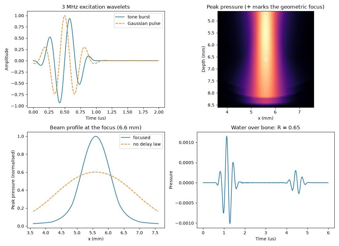
Laterally, a focused aperture localises sharply. The peak-pressure maximum – the largest pressure magnitude each cell ever sees, which is what a hydrophone scan reports – sits on the focal axis to within one cell, and the -6 dB beam width there is 21 cells, about twice the wavelength times the f-number. Removing the delay law widens it to 59 cells, roughly half the 120-cell aperture.
Axially, it does not, and no assertion should pretend otherwise. The depth of field of a focused aperture is about \(7\lambda F^2\) – around 70 cells for the \(F = 1\) aperture in the script – so the on-axis peak pressure is nearly flat right through the focal region, and its maximum lies well in front of the geometric focus: 24 cells short of it here, 20% of the focal length, and only 6% higher there than at the focus itself. That is ordinary physics, not a Deepwave artefact, and it is visible in the peak-pressure map below: the bright column is long, and brightest above the white cross. A time-integrated energy peak behaves the same way, only more so. An assertion that the peak-pressure maximum lands on the geometric focus would therefore be false in the axial direction, and one loosened until it passed would be measuring nothing.
What is sharp in the axial direction is the arrival time. The delay law’s whole purpose is that every element point’s contribution reaches the focus together, at max(range) / c after the wavelet’s own peak, and the script checks exactly that: the envelope of the trace recorded at the focal cell peaks within one cell of travel (\(\Delta x / c\), 0.033 µs here) of the predicted instant. Range is measured by time of flight, not by hunting for an amplitude maximum – in ultrasound as in seismic.
Fluid-solid interfaces (water and tissue over bone or rock)
Many ultrasound and seismic problems are fluid-solid: a fluid (water, or soft tissue modelled as a fluid) in contact with a solid that supports shear. Two common cases are transcranial ultrasound (water/soft tissue over the skull bone) and ocean-bottom seismic (a water column over the elastic seabed). The elastic propagator handles these directly: set the shear velocity vs = 0 in the fluid region (a fluid has no shear modulus, \(\mu = 0\)), and a non-zero vs in the solid. Build the Lamé/buoyancy models with deepwave.vpvsrho_to_lambmubuoyancy() as usual:
# Water over cortical bone. A fluid has no shear modulus, so its vs is 0;
# Deepwave's harmonic averaging of mu then imposes the fluid-solid
# condition (normal stress transmitted, no shear traction) for you.
vp_bone, vs_bone, rho_bone = 3.6, 1.8, 1.9  # mm/us, mm/us, and rho
interface = 100  # cells below the top of the model
ny_fs = 160 if smoke else 200
nx_fs = 121

vp = torch.full((ny_fs, nx_fs), v_water)
vs = torch.zeros(ny_fs, nx_fs)
rho = torch.full((ny_fs, nx_fs), rho_water)
vp[interface:] = vp_bone
vs[interface:] = vs_bone
rho[interface:] = rho_bone
lamb, mu, buoyancy = deepwave.vpvsrho_to_lambmubuoyancy(vp, vs, rho)

source_y, receiver_y, fs_x = 30, 50, nx_fs // 2
nt_fs = 600
fs_wavelet = gaussian_pulse(
    freq=freq,
    bandwidth_frac=0.6,
    nt=nt_fs,
    dt=dt,
    peak_time=peak_time,
    shape=(1, 1),  # [n_shots, n_sources, nt], with nothing copied
)
fs_out = elastic(
    lamb,
    mu,
    buoyancy,
    dx,
    dt,
    source_amplitudes_pressure_rate=fs_wavelet,
    source_locations_pressure_rate=torch.tensor([[[source_y, fs_x]]]),
    receiver_locations_p=torch.tensor([[[receiver_y, fs_x]]]),
    pml_width=pml_width,
    pml_freq=freq,
    accuracy=4,
)
fs_trace = fs_out.receiver_amplitudes_p[0, 0]
fs_envelope = envelope(fs_trace)

# Direct arrival and interface reflection, separated in time. Taking the
# *difference* of their arrival times cancels whatever time the source
# waveform itself takes to reach its peak.
direct_cells = receiver_y - source_y
reflect_cells = (interface - source_y) + (interface - receiver_y)
gap_samples = (reflect_cells - direct_cells) / c_cells / dt
split = round((direct_cells + reflect_cells) / 2 / c_cells / dt)
i_direct = int(fs_envelope[:split].argmax())
i_reflect = split + int(fs_envelope[split:].argmax())
gap_error = abs((i_reflect - i_direct) - gap_samples)

# The normal-incidence reflection coefficient, corrected for the
# 1/sqrt(range) spreading of a 2-D wave over the two path lengths.
spreading = math.sqrt(reflect_cells / direct_cells)
ratio = float(fs_envelope[i_reflect] / fs_envelope[i_direct])
r_measured = ratio * spreading
z_water = rho_water * v_water
z_bone = rho_bone * vp_bone
r_predicted = (z_bone - z_water) / (z_bone + z_water)
print(
    f"fluid-solid: reflection {i_reflect - i_direct} samples after the "
    f"direct arrival (predicted {gap_samples:.0f}); R = {r_measured:.3f} "
    f"(predicted {r_predicted:.3f})"
)

assert torch.isfinite(fs_trace).all(), "fluid-solid trace is not finite"
assert float(mu[:interface].abs().max()) == 0.0, (
    "the fluid region should carry no shear modulus"
)
assert gap_error <= 3, (
    f"the reflection arrived {gap_error:.0f} samples from its predicted "
    f"two-way time"
)
assert abs(r_measured - r_predicted) < 0.1 * r_predicted, (
    f"measured reflection coefficient {r_measured:.3f} is not within 10% "
    f"of the impedance-contrast prediction {r_predicted:.3f}"
)
Deepwave’s elastic parameter preparation evaluates the shear modulus at the staggered shear-stress nodes by a harmonic average of the surrounding cell values. Because the harmonic mean \(2\mu_1\mu_2/(\mu_1+\mu_2)\) goes to zero whenever either input is zero, every shear node that touches a fluid cell carries exactly zero shear modulus. That is precisely the physical fluid-solid condition: the interface transmits normal stress but no shear traction, and the fluid slips freely along the solid. This is imposed automatically; you only have to set vs = 0 in the fluid.
What is modelled correctly. At a fluid-solid interface an incident P wave splits into a reflected P (back into the fluid), a transmitted P, and – at oblique incidence – a mode-converted transmitted S wave in the solid. Deepwave reproduces the analytic behaviour: at normal incidence the reflection and transmission match the acoustic-impedance formulas \(R=(Z_1-Z_2)/(Z_1+Z_2)\) and \(T=2Z_1/(Z_1+Z_2)\) (using the solid’s P-impedance \(Z_2=\rho_2 v_{p2}\)) to a few percent – which is what the reflection check above measures, as a magnitude, after undoing the \(1/\sqrt{r}\) spreading of a 2-D wave over the two paths’ different lengths: 0.654 against the 0.640 the impedances predict – and at oblique incidence the reflected/transmitted-P/transmitted-S energy partition matches the fluid-solid Zoeppritz solution to ~1-2% (validated in tests/test_elastic_fluid_solid.py).
Stability and near-interface oscillations. A water layer over a solid with a free surface on top (the ocean-bottom, or a water-coupled ultrasound tank geometry) is long-run stable in Deepwave. Unlike the thin-slab-between-two- free-surfaces case (see Boundary conditions), the water’s lower boundary is a fluid-solid interface rather than a second free surface, so the elastic C-PML instability condition is not met. If you see oscillations in traces recorded near the interface (as reported in Deepwave issue #116), these are a near-interface numerical/physical effect – Scholte interface waves and grid dispersion – not a divergence. To reduce them, increase the points per wavelength near the interface (finer grid_spacing or higher accuracy), and avoid placing receivers on the interface row itself; place them a cell or two into the medium you want to record. See Troubleshooting.
The figure
The last section of the script plots the two wavelets, the peak-pressure map around the focus, the focused and unfocused beam profiles at the focal depth, and the water-over-bone trace:
time_axis = torch.arange(nt_wavelet) * dt
extent = [
    float(patch_x[0]) * dx,
    float(patch_x[-1]) * dx,
    float(patch_y[-1]) * dx,
    float(patch_y[0]) * dx,
]
_, ax = plt.subplots(2, 2, figsize=(11, 8))
ax[0, 0].plot(time_axis, burst, label="tone burst")
ax[0, 0].plot(time_axis, pulse, "--", label="Gaussian pulse")
ax[0, 0].set_xlabel("Time (us)")
ax[0, 0].set_ylabel("Amplitude")
ax[0, 0].set_title(f"{freq:g} MHz excitation wavelets")
ax[0, 0].legend()

ax[0, 1].imshow(peak_focused, extent=extent, cmap="magma", aspect="equal")
ax[0, 1].plot(centre_x * dx, focus_y * dx, "w+", markersize=12)
ax[0, 1].set_xlabel("x (mm)")
ax[0, 1].set_ylabel("Depth (mm)")
ax[0, 1].set_title("Peak pressure (+ marks the geometric focus)")

peak_scale = lateral_focused.max()
ax[1, 0].plot(patch_x * dx, lateral_focused / peak_scale, label="focused")
ax[1, 0].plot(
    patch_x * dx,
    lateral_unfocused / peak_scale,
    "--",
    label="no delay law",
)
ax[1, 0].set_xlabel("x (mm)")
ax[1, 0].set_ylabel("Peak pressure (normalised)")
ax[1, 0].set_title(f"Beam profile at the focus ({focus_y * dx:g} mm)")
ax[1, 0].legend()

ax[1, 1].plot(torch.arange(nt_fs) * dt, fs_trace)
ax[1, 1].set_xlabel("Time (us)")
ax[1, 1].set_ylabel("Pressure")
ax[1, 1].set_title(f"Water over bone: R = {r_measured:.2f}")

plt.tight_layout()
plt.savefig("example_ultrasound.jpg")
plt.show()
Honest differences from k-Wave
k-Wave is a mature, ultrasound-specialised package, and there are things it does that Deepwave does not (yet):
Numerical method. Deepwave is a finite-difference code on a regular Cartesian grid, so curved boundaries and off-axis transducer surfaces are represented by staircased/interpolated points, whereas k-Wave’s k-space pseudospectral method needs far fewer points per wavelength and has no grid dispersion of the same kind. For the same accuracy Deepwave typically needs a finer grid.
Tissue absorption. k-Wave natively models power-law frequency-dependent absorption, the standard soft-tissue attenuation model. Deepwave provides
deepwave.viscoacoustic, a constant-Q, single-mechanism standard-linear-solid (SLS) propagator: you supply a quality factorQat a reference frequencyq_freqand get (approximately) constant-Q attenuation near that frequency. What is still missing is k-Wave’s power-law frequency-dependent absorption model itself; fitting a power law over a wide band with multiple SLS mechanisms remains future work (roadmap). Until then, use a single SLS mechanism tuned near your dominant frequency, or model lossless propagation.
What Deepwave offers in return is full differentiability: gradients of any output with respect to the sound-speed/density model, the source wavelet, the initial pressure, apodisation, and focusing delays, computed to machine precision through compiled kernels (with true second-order Hessian-vector products for the scalar propagator). That turns imaging and characterisation problems – photoacoustic reconstruction, transcranial aberration correction, sound-speed tomography, transducer/delay-law design – into ordinary PyTorch optimisation, on CPU or GPU, composable with any torch loss or neural network. k-Wave is not differentiable.
Note
Precision on long ultrasound runs. Ultrasound simulations often use many thousands of time steps (high sample rates over long records). In float32 the small per-step rounding errors accumulate, and phase drift can become visible late in a long run. If you see this, run in float64 (pass float64 model/source tensors) for a reference, or verify that float32 phase error is acceptable for your record length; float32 is usually fine for imaging but worth checking for quantitative timing measurements. This is the same accumulation caveat noted for the eager backend in Accuracy and grid design.
See also
Photoacoustic initial-pressure reconstruction – a worked differentiable photoacoustic reconstruction.
Units and source conventions – the source/receiver amplitude conventions per propagator.
Boundary conditions – edge conditions, including the first-class
boundaryselector for free (pressure-release, e.g. a water/air interface), rigid, and periodic faces.Choosing a wave-propagation package – how Deepwave compares with k-Wave and other packages.