Q (attenuation) inversion with the viscoacoustic propagator

deepwave.viscoacoustic() models a quality factor Q per grid cell using generalised-standard-linear-solid (GSLS) relaxation mechanisms (see Viscoacoustic (attenuating) wave equation). Passing q_n_mechanisms > 1 together with a q_band fits several relaxation mechanisms so that Q is close to constant across a whole frequency band, rather than exact only at one reference frequency – this example uses two mechanisms across a 10-50 Hz band. There is then no single reference frequency, so q_freq is not given (a single-mechanism call must give it). The anomalous target q=20 produces an actual \(Q_{\mathrm{eff}}\approx 21.05\) at the 25 Hz wavelet frequency in this two-mechanism fit. The example prints this value using deepwave.attenuation.response(); other frequencies have a different response.

A small crosswell-style survey images a localised low-Q (highly attenuating) anomaly on top of an otherwise nearly-elastic (high-Q) background, starting from a uniform high-Q guess:

out = viscoacoustic(
    v, rho, q, dx, dt,
    source_amplitudes_pressure_rate=source_amplitudes,
    source_locations_pressure_rate=source_locations,
    receiver_locations_p=receiver_locations,
    q_n_mechanisms=2,
    q_band=(10.0, 50.0),
    pml_freq=freq,
    max_vel=3000.0,
)

Q is inverted with q = 10 + exp(logq), keeping it above 10, using the same chain-rule reparameterisation pattern as FWI in other parameterisations. This example also applies the masked-subregion pattern from Model parameterisations: only a central region away from the sources and the PML is optimised, since this small survey’s limited illumination there produces inversion artefacts if the whole model is left free to update:

invert_mask = (yy > 8) & (xx > 8) & (xx < nx - 8)
update = torch.zeros((ny, nx), requires_grad=True)

for _epoch in range(n_epochs):
    optimiser.zero_grad()
    logq = logq_background + torch.where(
        invert_mask, update, torch.zeros_like(update)
    )
    q = 10.0 + torch.exp(logq)
    loss = loss_fn(run(q) / data_scale, observed / data_scale)
    loss.backward()
    optimiser.step()

The pressure-rate wavelet has a peak amplitude of \(10^6\) Pa/s. data_scale is the fixed RMS amplitude of the observed data, so loss normalisation keeps the optimiser’s scale independent of the source units. The fixed max_vel bounds the unrelaxed speed over this example’s allowed Q range; using v.max() would only bound the relaxed speed.

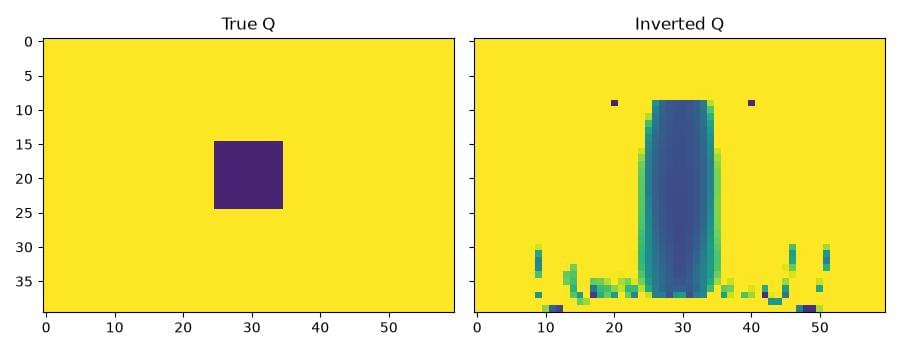
This small survey recovers a low-Q band near the anomaly’s lateral position, with substantial vertical smearing and additional artefacts. The decrease in data misfit demonstrates differentiation and optimisation; it does not establish a unique reconstruction or accurate recovery of the anomaly’s depth extent. A better-resolved inversion needs more illumination and appropriate regularisation.

Full example code