Full-Waveform Inversion of a portion of Marmousi
Full-Waveform Inversion provides the potential to invert for a model that matches the whole wavefield, including refracted arrivals. It performs inversion using the regular propagator rather than the Born propagator.
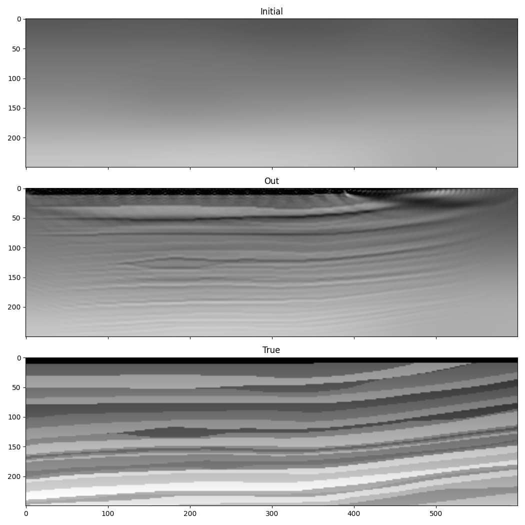
We continue with using the Marmousi model, but due to the computational cost of running many iterations of FWI, we will work on only a portion of it:
import torch
from scipy.ndimage import gaussian_filter
import matplotlib.pyplot as plt
import deepwave
from deepwave import scalar

device = torch.device('cuda' if torch.cuda.is_available()
                      else 'cpu')
ny = 2301
nx = 751
dx = 4.0
v_true = torch.from_file('marmousi_vp.bin',
                         size=ny*nx).reshape(ny, nx)

# Select portion of model for inversion
ny = 600
nx = 250
v_true = v_true[:ny, :nx]
We smooth the true model to create our initial guess of the wavespeed, which we will attempt to improve with inversion. We also load the data that we generated in the forward modelling example to serve as our target observed data:
v_init = (torch.tensor(1/gaussian_filter(1/v_true.numpy(), 40))
          .to(device))
v = v_init.clone()
v.requires_grad_()

n_shots = 115

n_sources_per_shot = 1
d_source = 20  # 20 * 4m = 80m
first_source = 10  # 10 * 4m = 40m
source_depth = 2  # 2 * 4m = 8m

n_receivers_per_shot = 384
d_receiver = 6  # 6 * 4m = 24m
first_receiver = 0  # 0 * 4m = 0m
receiver_depth = 2  # 2 * 4m = 8m

freq = 25
nt = 750
dt = 0.004
peak_time = 1.5 / freq

observed_data = (
    torch.from_file('marmousi_data.bin',
                    size=n_shots*n_receivers_per_shot*nt)
    .reshape(n_shots, n_receivers_per_shot, nt)
)
As our model is now smaller, we also need to extract only the portion of the observed data that covers this section of the model:
n_shots = 20
n_receivers_per_shot = 100
nt = 300
observed_data = (
    observed_data[:n_shots, :n_receivers_per_shot, :nt].to(device)
)
We set-up the sources and receivers as before:
# source_locations
source_locations = torch.zeros(n_shots, n_sources_per_shot, 2,
                               dtype=torch.long, device=device)
source_locations[..., 1] = source_depth
source_locations[:, 0, 0] = (torch.arange(n_shots) * d_source +
                             first_source)

# receiver_locations
receiver_locations = torch.zeros(n_shots, n_receivers_per_shot, 2,
                                 dtype=torch.long, device=device)
receiver_locations[..., 1] = receiver_depth
receiver_locations[:, :, 0] = (
    (torch.arange(n_receivers_per_shot) * d_receiver +
     first_receiver)
    .repeat(n_shots, 1)
)

# source_amplitudes
source_amplitudes = (
    (deepwave.wavelets.ricker(freq, nt, dt, peak_time))
    .repeat(n_shots, n_sources_per_shot, 1).to(device)
)
We are now ready to run the optimiser to perform iterative inversion of the wavespeed model. We apply a scaling (1e10) to boost the gradient values to a range that will help us to make good progress with each iteration, but also apply a clipping to the gradients (to the 98th percentile of their magnitude) to avoid making very large changes at a small number of points (such as around the sources):
# Setup optimiser to perform inversion
optimiser = torch.optim.SGD([v], lr=0.1, momentum=0.9)
loss_fn = torch.nn.MSELoss()

# Run optimisation/inversion
n_epochs = 250
v_true = v_true.to(device)

for epoch in range(n_epochs):
    def closure():
        optimiser.zero_grad()
        out = scalar(
            v, dx, dt,
            source_amplitudes=source_amplitudes,
            source_locations=source_locations,
            receiver_locations=receiver_locations,
            pml_freq=freq,
        )
        loss = 1e10 * loss_fn(out[-1], observed_data)
        loss.backward()
        torch.nn.utils.clip_grad_value_(
            v,
            torch.quantile(v.grad.detach().abs(), 0.98)
        )
        return loss

    optimiser.step(closure)
The result is quite a good improvement in the accuracy of our estimate of the wavespeed model.
This is a simple implementation of FWI. Faster convergence and greater robustness in more realistic situations can be achieved with modifications such as a more sophisticated loss function. You can find some slightly more sophisticated setups in some of the other examples, and Deepwave makes it easy for you to come-up with your own. As PyTorch will automatically backpropagate through any differentiable operations that you apply to the output of Deepwave, you only have to specify the forward action of such loss functions and can then let PyTorch automatically handle the backpropagation.