FWI in other parameterisations

Every Deepwave propagator takes physical model tensors directly (wavespeed, density, stiffnesses, …) and every output is differentiable with respect to them. But the tensor you hand a propagator does not have to be the tensor you optimise. Because propagation is an ordinary PyTorch operation, any invertible reparameterisation built from plain tensor arithmetic composes with autograd automatically: build the propagator’s native inputs from your own optimised variables inside the loss, call the propagator, and backward() chains the gradient through your reparameterisation for free.

This is worth stating explicitly because some other packages advertise specific parameterisations (e.g. “impedance FWI”) as if they needed dedicated physics or a special API. In Deepwave they don’t: any parameterisation – impedance, log-velocity, slowness, a neural-network reparameterisation, a physically-constrained transform – is available via plain PyTorch, with no propagator-side support required. (See also Choosing a wave-propagation package, which makes the same point about reparameterisations in general; this page gives the worked recipe.)

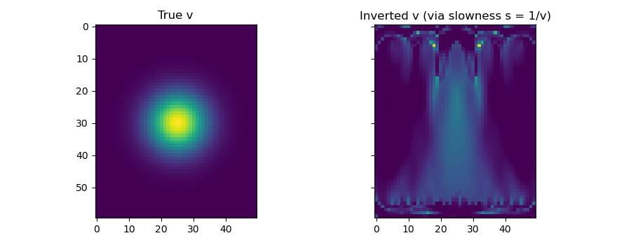
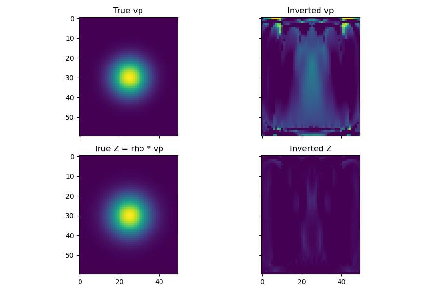
Both sections below run the same small crosswell survey (sources down the left edge, receivers down the right, so the modelled waves transmit through the anomaly) and start from a homogeneous model with no knowledge of the anomaly’s location – a deliberately hard, minimal setup, so the recovered images are recognisable but not pixel-perfect.

Acoustic: velocity/impedance parameterisation

For the variable-density acoustic propagator, deepwave.acoustic() takes (vp, rho). To instead optimise velocity and impedance \(Z = \rho v_p\) directly, keep vp and Z as the leaf tensors and rebuild rho from them every iteration before calling the propagator:

vp = (1500.0 * torch.ones(ny, nx)).requires_grad_()
Z = (1500.0 * 2200.0 * torch.ones(ny, nx)).requires_grad_()
optimizer = torch.optim.Adam(
    [{"params": [vp], "lr": 9.0}, {"params": [Z], "lr": 3500.0}]
)

for _epoch in range(n_epochs):
    optimizer.zero_grad()
    rho = Z / vp
    loss = torch.nn.functional.mse_loss(
        run_acoustic(vp, rho), observed_p
    )
    loss.backward()
    optimizer.step()

rho = Z / vp is the entire “impedance equation”: a division, not a new propagator mode. vp.grad and Z.grad are exactly what the chain rule gives for \(\partial\text{loss}/\partial v_p\) and \(\partial\text{loss}/\partial Z\) through that division – note the two parameters need very different learning rates because they live on very different physical scales (velocity in m/s, impedance in Pa*s/m), an ordinary optimiser-tuning concern rather than anything specific to reparameterised FWI.

Scalar: slowness parameterisation

The same recipe applies to any other invertible transform. For the constant- density scalar propagator, optimising slowness \(s = 1/v_p\) –the natural variable in traveltime tomography– instead of velocity is a one-line change: keep s as the leaf tensor and rebuild v = 1 / s before the call:

s = (1.0 / (1500.0 * torch.ones(ny, nx))).requires_grad_()
optimizer = torch.optim.Adam([s], lr=3e-6)

for _epoch in range(n_epochs):
    optimizer.zero_grad()
    loss = torch.nn.functional.mse_loss(run_scalar(1.0 / s), observed)
    loss.backward()
    optimizer.step()

A log-velocity parameterisation (logv = torch.log(v0), rebuilding v = torch.exp(logv)) is exactly as simple, and has the added benefit that v is guaranteed positive for any logv – again, ordinary PyTorch, not a propagator feature.

Full example code