Earthquake (moment tensor) sources
Deepwave’s elastic propagator takes body forces: you tell it how hard to push, in which direction, and where. Earthquake seismologists do not describe a source that way. They describe it with a moment tensor. This page shows how to turn a moment tensor into the body forces Deepwave wants. No new Deepwave function is needed. The recipe is ordinary user code, and it is verified here against the radiation pattern that theory predicts.
What a moment tensor is
An earthquake is slip on a fault: two blocks of rock slide past each other. Nothing pushes the Earth from outside, so the source exerts no net force. What it does exert is pairs of opposing forces. A pair of opposing forces is called a couple.
The moment tensor collects those couples. It is a symmetric 3x3 tensor. Its component \(M_{ij}\) is the strength of a couple made of two opposing forces that point along direction \(i\) and are separated by a small distance along direction \(j\). Because the tensor is symmetric, \(M_{ij} = M_{ji}\), and the source has no net torque either. Each component has units of force times length (newton metres in SI).
The scalar moment, written \(M_0\), is the size of the earthquake. For slip on a fault it is the shear modulus times the area that slipped times the average amount of slip. Earthquake magnitudes are computed from it.
Slip on a plane gives a particular kind of moment tensor called a double couple: two couples of equal strength, at right angles to each other. An explosion gives a different one: an isotropic moment tensor, equal to \(M_0\) times the identity, which pushes outwards equally in all directions. Both appear below.
The orientation of a fault and the direction of slip on it are given by three angles.
Strike is the compass direction of the fault’s horizontal trace, measured clockwise from North. The fault dips down to the right of the strike direction.
Dip is the angle of the fault plane below horizontal, from 0 (horizontal) to 90 degrees (vertical).
Rake is the direction the rock slipped, measured within the fault plane, anticlockwise from the strike direction. A rake of 0 is horizontal (strike slip); 90 is the upper block riding up the fault (reverse, or thrust, slip); -90 is the upper block sliding down (normal slip).
From strike, dip and rake to the moment tensor
The relations used here are those of Aki and Richards, Quantitative Seismology: Theory and Methods (W. H. Freeman, 1980). They are written in a right-handed Cartesian frame whose axes are North, East and Down, so depth increases along the third axis.
In that frame the unit vector along the slip direction and the unit vector normal to the fault plane are both fixed by the three angles. The moment tensor of a shear dislocation is then the symmetric outer product of the two, scaled by the scalar moment:
slip = torch.tensor([
    math.cos(rake_rad) * math.cos(strike_rad)
    + math.cos(dip_rad) * math.sin(rake_rad) * math.sin(strike_rad),
    math.cos(rake_rad) * math.sin(strike_rad)
    - math.cos(dip_rad) * math.sin(rake_rad) * math.cos(strike_rad),
    -math.sin(rake_rad) * math.sin(dip_rad),
])
normal = torch.tensor([
    -math.sin(dip_rad) * math.sin(strike_rad),
    math.sin(dip_rad) * math.cos(strike_rad),
    -math.cos(dip_rad),
])
moment_tensor = m0 * (
    torch.outer(slip, normal) + torch.outer(normal, slip)
)
(the three angles are in radians here). The example also writes out the six components one by one, in the form the relations are usually quoted in, and asserts that the two forms agree. That is worth doing once in your own code: a sign slip in one component is otherwise easy to miss.
Mapping the frame onto Deepwave’s grid
Deepwave orders its spatial dimensions from slowest to fastest varying: (z, y, x) in 3-D and (y, x) in 2-D. It attaches no physical meaning to them, so you choose what they mean (see Units and source conventions). The example is a 2-D vertical cross-section, and takes
Deepwave
y, the first dimension, to be Down (depth),Deepwave
x, the second dimension, to be North.
Selecting the rows and columns of the moment tensor that belong to those two axes gives the 2-D moment tensor:
in_plane = [2, 0]  # (Down, North)
moment_tensor_2d = moment_tensor[in_plane][:, in_plane]
A 2-D simulation carries only motion in the model plane: P waves, and the S waves whose motion is polarised in that plane (SV waves). The components of the moment tensor that involve the out-of-plane axis drive S waves polarised out of the plane (SH waves), which the 2-D simulation does not model, so they are dropped. To keep every component meaningful, the example chooses a fault that strikes East-West, so that the North-Down cross-section is perpendicular to the strike and contains both the slip vector and the fault normal. Note also that a 2-D source is a line source, uniform and infinite out of the plane, so \(M_0\) is really a moment per unit length out of the plane.
From moment tensor to body force couples
A point moment tensor source at position \(\mathbf{s}\) is equivalent to the body force density
which is the couple description written as mathematics: the force in direction \(i\) is a derivative, along direction \(j\), of a point source of strength \(M_{ij}\). Three practical consequences follow.
Two forces, opposite signs. A derivative is approximated by a difference, so each component becomes two point forces straddling the source position: \(+M_{ij}\) on the \(+j\) side and \(-M_{ij}\) on the \(-j\) side.
Divide by the separation. A difference only approximates a derivative after dividing by the step. The example puts the two forces half a cell either side of the source, so their separation, the lever arm, is one cell, dx.
Divide by the cell volume. Deepwave’s velocity sources are force densities, in units of force per volume (see Units and source conventions). A point force of \(F\) newtons applied in one cell is a density of \(F\) divided by the cell volume. In 2-D that volume is dx * dx per unit length out of the plane.
The last thing to respect is where each force may be applied. On the staggered grid (see Elastic wave equation) the field components do not share a position: the normal stresses and the model parameters sit on the integer grid points \((y, x)\), while \(v_y\) sits at \((y+\frac{1}{2}, x)\) and \(v_x\) at \((y, x+\frac{1}{2})\). A force in the y direction is applied to \(v_y\), so it can only act where \(v_y\) lives.
You do not have to do that bookkeeping by hand. Location arguments given as floating point numbers are physical positions in grid cells, and Deepwave removes each component’s own half-cell offset for you (see the section on off-grid sources and receivers in Usage). A position that lands exactly on that component’s node is injected exactly; one that falls between nodes is interpolated with a windowed sinc. So the four positions can simply be written down as the physical offsets they are:
separation = torch.tensor(
    [[0.5, 0.0], [-0.5, 0.0], [0.0, 0.5], [0.0, -0.5]]
)
couple_locations = source_position + separation

weights_y = torch.tensor(
    [moment[0, 0], -moment[0, 0], moment[0, 1], -moment[0, 1]]
)
weights_x = torch.tensor(
    [moment[1, 0], -moment[1, 0], moment[1, 1], -moment[1, 1]]
)
scale = 1.0 / (lever_arm * cell_volume)
The first two positions are separated along y and carry the \(M_{yy}\) and \(M_{xy}\) couples; the second two are separated along x and carry \(M_{yx}\) and \(M_{xx}\). The same four positions serve both force directions, with different weights, and both are passed to deepwave.elastic() as ordinary sources:
out = elastic(
    lamb, mu, buoyancy, dx, dt,
    source_amplitudes_y=amplitudes_y,
    source_locations_y=couple_locations,
    source_amplitudes_x=amplitudes_x,
    source_locations_x=couple_locations,
    receiver_locations_y=receiver_locations,
    receiver_locations_x=receiver_locations,
    pml_width=pml_width, pml_freq=freq,
)
One point about time is easy to overlook. The amplitudes above are proportional to the moment \(M(t)\) itself, not to its rate of change. If you have a moment rate function, integrate it first.
Checking the sign and the scale
Getting the sign of the couples backwards turns an explosion into an implosion, and nothing about the shape of the wavefield will tell you. The example therefore pins the sign and the scale down independently. It applies the same recipe to an isotropic moment tensor, which is an explosion, and compares the result with Deepwave’s own explosive source (the pressure_rate channel). The body force has an equivalent description as a stress glut: it adds \(-M_{ij}\delta(\mathbf{x}-\mathbf{s})\) to the stress. For an isotropic moment tensor \(M_0 w(t)\), and since pressure is minus the mean normal stress, that is a pressure of \(M_0 w(t)\) spread over one cell. Deepwave’s pressure source is specified as a pressure rate (see Units and source conventions), so the equivalent amplitude is the time derivative of that, \(M_0 \dot{w}(t)\) divided by the cell volume. The two runs agree to 0.3% in amplitude, and in sign.
Verifying the radiation pattern
The radiation pattern of a source is the way the amplitude it radiates varies with direction. For P waves in the far field it is the moment tensor contracted twice with the unit vector \(\boldsymbol{\gamma}\) that points from the source to the receiver: the amplitude is proportional to \(\gamma_i M_{ij} \gamma_j\). For a double couple this equals \(2 M_0 (\boldsymbol{\gamma}\cdot\mathbf{s}) (\boldsymbol{\gamma}\cdot\mathbf{n})\), with \(\mathbf{s}\) the slip vector and \(\mathbf{n}\) the fault normal.
That form makes the classic picture immediate. The pattern has four lobes. It is positive (the first ground motion is away from the source, a compression) in two opposite quadrants, and negative (the first motion is towards the source, a dilatation) in the other two. It vanishes on two perpendicular planes, called nodal planes, where \(\boldsymbol{\gamma}\) is perpendicular to the slip vector or to the fault normal. Those two planes are the fault plane itself and the plane perpendicular to the slip, which is called the auxiliary plane. P-wave first motions alone cannot tell you which of the two is the real fault: this is the classic fault plane ambiguity.
The example measures the pattern. Receivers are placed on a circle around the source, five P wavelengths away, far enough for the far-field form to have developed. Both velocity components are recorded at each receiver and projected onto the source-receiver direction, giving the radial velocity. Because every receiver is the same distance from the source, the P arrival has the same shape at all of them and differs only by a scale factor, which is exactly the radiation pattern. Projecting each receiver’s trace onto the explosion run’s waveform, over a window that opens at the P travel time and closes at the S travel time, therefore measures the pattern directly, and in absolute units, because the explosion radiates \(M_0\) in every direction:
window = (time >= radius * dx / vp) & (time <= radius * dx / vs)
reference = radial_explosion[:, window].mean(dim=0)
measured = (
    (radial_double_couple[:, window] * reference).sum(dim=1)
    / (reference * reference).sum()
)
predicted = torch.einsum(
    "ai,ij,aj->a", direction, moment_tensor_2d / m0, direction
)
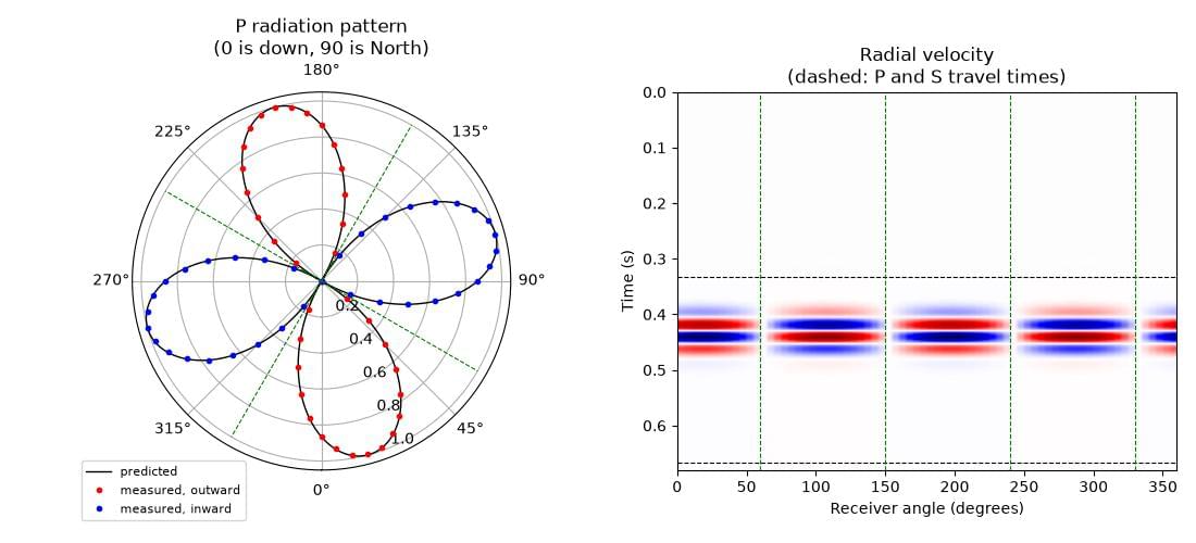
The left panel is the measured pattern (points, coloured by whether the first motion is outward or inward) on top of the prediction (line), with the predicted nodal directions dashed. The right panel is the radial velocity recorded around the circle: the polarity of the P arrival reverses as each nodal direction is crossed, which is the same information in a different form.
For a fault striking East-West, dipping at 60 degrees, with pure reverse slip, the measured pattern differs from the prediction by at most 0.006 of the peak amplitude, the measured amplitude at each of the four predicted nodal directions is below 0.001 of the peak, and the polarity agrees with the prediction at every receiver that is not close to a nodal direction (where the predicted amplitude is above a fifth of the peak, so that “polarity” means something). The example asserts all of this, so it fails if the recipe or the propagator stops reproducing the theory.
The residual difference is not noise. It has two causes, and both can be made smaller. The first is the finite grid: a couple built from two forces one cell apart is only a second-order accurate approximation of a derivative. Its size is visible in the comparison with Deepwave’s explosive source, which improves from 1.3% at a grid spacing of 20 m, to 0.3% at 10 m, to 0.07% at 5 m – a quarter of the error for each halving, as second-order accuracy predicts. The second is the finite distance to the receivers: “far field” means infinitely far, and at five wavelengths the near-field terms have not entirely died away. Moving the circle out to ten and then fifteen wavelengths reduces the largest difference from 0.006 to 0.004 and then 0.003.