FWI Recipes: Exotic Misfits, Deep Priors, and Uncertainty
Competing differentiable-FWI packages often advertise a long list of “batteries-included” features: optimal-transport and soft-DTW misfit functions, deep-image-prior network reparameterisation, and dropout-based uncertainty quantification. The point of this example is that, because Deepwave is just a differentiable forward modelling operator that plugs into the stock PyTorch ecosystem, each of those features is a short recipe rather than a new API surface. You compose them; Deepwave does not need to provide them.
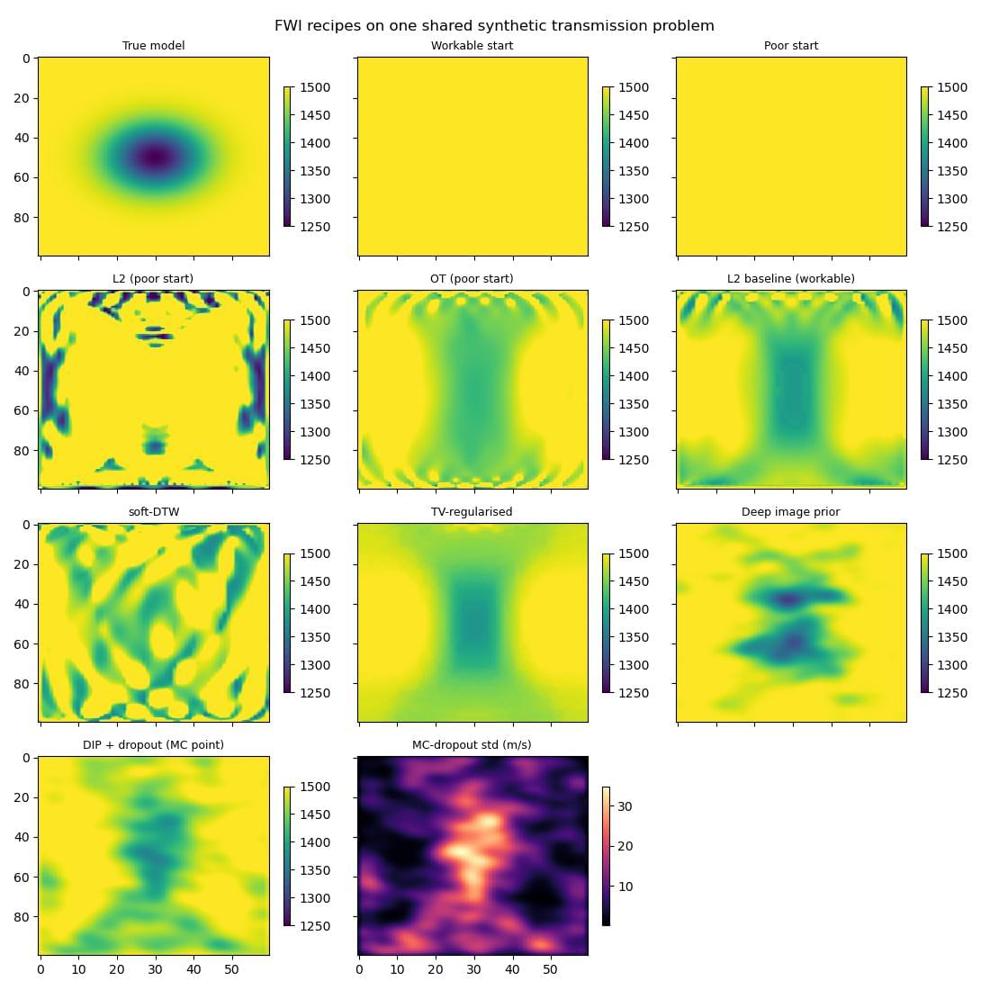
To keep the comparison honest, every recipe shares one small, self-contained 2-D synthetic problem. The true model is a constant 1500 m/s background with a Gaussian low-velocity anomaly (down to ~1250 m/s). The acquisition is a cross-hole transmission geometry: eight sources down the left edge, thirty receivers down the right edge, so the wave transmits through the anomaly and its arrival time carries the signal. From this single problem we derive two homogeneous starting models:
a poor start (1600 m/s everywhere — too fast, so the whole transmitted wavetrain is time-shifted) that exposes cycle-skipping. It drives the optimal-transport recipe, where plain least-squares fails and transport-based misfits recover.
a workable start (the correct 1500 m/s background, so only the anomaly is unknown) that drives the soft-DTW, deep-image-prior, dropout-uncertainty, and regularisation recipes, which are about ill-posedness and prior information rather than cycle-skipping.
The script runs every recipe end-to-end, prints a metrics table (model RMSE in m/s and a common L2 data misfit per recipe), and writes one comparison figure. Each recipe below shows only its core excerpt; see the full script for the shared setup and plotting.
Recipe 1: the L2 baseline
The reference against which everything else is judged is ordinary least-squares FWI: optimise the velocity pixels directly to minimise the mean-squared error between predicted and observed traces. In Deepwave this is the loop you have already seen in the other examples:
def invert_pixels(loss_fn, v_start, n_epochs=60, lr=6.0):
    v = v_start.clone().requires_grad_()
    opt = torch.optim.Adam([v], lr=lr)
    for _ in range(n_epochs):
        opt.zero_grad()
        loss_fn(forward(v)).backward()
        opt.step()
    return v.detach()
From the workable start this recovers the anomaly well, and it is the yardstick for the regularisation recipes. From the poor start the same L2 loss cycle-skips badly (see Recipe 2).
Recipe 2: optimal-transport (Wasserstein) misfit
The classic cure for cycle-skipping is a misfit that measures time shift, not just amplitude mismatch. Optimal transport does exactly this: the Wasserstein-2 distance between two signals, viewed as mass distributions over time, grows like the squared shift between them — a convex penalty far less prone to the spurious local minima that trap L2 (Engquist & Froese 2014; Métivier et al. 2016).
Two subtleties matter, and the example handles both explicitly:
Signed data. Transport needs non-negative mass, but seismograms swing positive and negative. We map each trace to an energy density over time,
p(t) = a(t)^2 / sum_t a(t)^2. Squaring makes the mass non-negative and emphasises energetic arrivals; normalising makes each trace a probability measure, so predicted and observed mass match (balanced OT). The price is that squaring discards polarity — this is a phase-insensitive, envelope-like comparison.The ground cost is squared time distance, so a shifted arrival costs approximately
shift^2.
def energy_density(traces):
    """Map signed traces (B, nt) to non-negative densities over time."""
    energy = traces**2
    energy = energy + 1e-6 * energy.mean(dim=-1, keepdim=True)
    return energy / energy.sum(dim=-1, keepdim=True)
For the transport distance itself the example uses geomloss when it is installed (an optional dependency included in deepwave[examples], not required by Deepwave itself), falling back to a pure-torch implementation otherwise. The import is guarded so the script runs either way:
try:
    from geomloss import SamplesLoss

    HAVE_GEOMLOSS = True
except ImportError:
    HAVE_GEOMLOSS = False
Why the fallback exists, and what it is. geomloss runs happily CPU-only here with its "tensorized" backend, so it is the default. But most Deepwave users will not have it installed, and for 1-D distributions we do not need a general entropic solver at all: the squared Wasserstein-2 distance between two 1-D densities is the squared L2 distance between their quantile (inverse-CDF) functions (Métivier et al. 2016). That is a few lines of pure PyTorch. The example approximates that integral using sampled, linearly interpolated quantiles; it has no entropic regularisation, but it still has interpolation and quadrature error.
The interpolation is essential for inversion. Indexing a constant time axis with torch.searchsorted alone disconnects the loss from the predicted amplitudes. Here searchsorted selects a bracket, and the interpolated value retains a gradient through the CDF samples:
def _quantile(cdf, levels, t):
    """Differentiable inverse-CDF (quantile) via linear interpolation.

    ``torch.searchsorted`` only selects which pair of CDF samples brackets
    each level; that index choice is a discrete, non-differentiable
    decision (as with nearest-bin lookups generally) and does not need a
    gradient. The quantile *value* is then linearly interpolated between
    the bracketing ``(t, cdf)`` samples, so it is a differentiable function
    of ``cdf`` (and therefore of whatever produced it, e.g. ``pred``).
    """
    idx = torch.searchsorted(cdf, levels).clamp(1, cdf.shape[-1] - 1)
    cdf_hi = torch.gather(cdf, -1, idx)
    cdf_lo = torch.gather(cdf, -1, idx - 1)
    t_hi = t[idx]
    t_lo = t[idx - 1]
    frac = (levels - cdf_lo) / (cdf_hi - cdf_lo).clamp_min(1e-12)
    return t_lo + frac * (t_hi - t_lo)
The complete fallback uses the example’s pooling factor and time axis:
def cdf_wasserstein(pred, target):
    """Pure-torch 1-D W2 via inverse-CDF (geomloss-free fallback).

    For 1-D distributions the squared Wasserstein-2 distance is the
    squared L2 distance between the quantile (inverse-CDF) functions
    (Metivier et al. 2016). We sample the quantile axis uniformly and read
    off the arrival *time* at each quantile of the energy density.

    The quantile lookup must be done with :func:`_quantile`, not plain
    ``t[torch.searchsorted(cdf, levels)]`` indexing: gathering ``t`` (a
    constant time axis) at the integer indices returned by
    ``torch.searchsorted`` (also non-differentiable) leaves the result with
    no path back to ``cdf`` at all, so ``pred``'s gradient is silently
    dropped and ``loss.backward()`` raises "does not require grad" instead
    of quietly producing a wrong (zero) gradient.
    """
    p = energy_density(decimate(pred, ot_time_factor).reshape(-1, nt_ot))
    q = energy_density(decimate(target, ot_time_factor).reshape(-1, nt_ot))
    cp = torch.cumsum(p, dim=-1)
    cq = torch.cumsum(q, dim=-1)
    levels = torch.linspace(0.0, 1.0, nt_ot, device=device).expand(
        cp.shape[0], -1
    )
    t = ot_time_axis.reshape(nt_ot)
    qp = _quantile(cp, levels, t)
    qq = _quantile(cq, levels, t)
    return ((qp - qq) ** 2).mean()
Both paths tell the same story. From the poor start, L2 cycle-skips into a model that is worse than the starting guess, whereas the transport-based misfit relaxes the arrival-time mismatch and recovers a model close to the truth. The metrics table quantifies the gap.
Recipe 3: a compact soft-DTW misfit
Soft dynamic time warping (Cuturi & Blondel 2017) is a second time-shift-tolerant misfit. It is the classic dynamic-time-warping recursion with the hard min replaced by a log-sum-exp soft minimum (temperature gamma), which makes it smooth and differentiable. Unlike the energy-density OT above it keeps polarity. The whole thing is about forty lines of pure PyTorch:
def soft_dtw(x, y, gamma=0.1):
    """Soft-DTW discrepancy between batches of 1-D series (B, T)."""
    n, t_len = x.shape
    dist = (x.unsqueeze(2) - y.unsqueeze(1)) ** 2  # (B, T, T)
    big = x.new_full((n,), 1e10)
    prev = [x.new_zeros(n)] + [big] * t_len  # previous row, j = 0..T
    for i in range(1, t_len + 1):
        curr = [big]  # j = 0 boundary is +inf
        for j in range(1, t_len + 1):
            neighbours = torch.stack(
                [prev[j], curr[j - 1], prev[j - 1]]
            )
            soft_min = -gamma * torch.logsumexp(
                -neighbours / gamma, dim=0
            )
            curr.append(dist[:, i - 1, j - 1] + soft_min)
        prev = curr
    return prev[t_len]
The dynamic program is O(T^2) per trace pair, so the example subsamples the traces in time and space and compares per-trace normalised waveforms (shape, not amplitude). We accumulate the cost matrix one row at a time into small per-cell tensors rather than assigning into one big tensor in place; that keeps the autograd graph cheap to backprop, which matters because the misfit is evaluated every FWI iteration.
Two honesty caveats. The script prints soft-DTW against a progressively time-shifted Ricker wavelet, next to L2. L2 oscillates — a larger shift can score lower than a smaller one, which is exactly cycle-skipping — whereas soft-DTW is a monotone bowl that grows with the shift. But (1) raw soft-DTW is not a true metric: the soft minimum is biased below the hard minimum, so the values carry a negative offset and D(x, x) != 0. The non-negative soft-DTW divergence of Blondel et al. 2020 subtracts the self-terms to fix this; we keep the raw form for brevity and simply note the minimum still sits at zero shift. And (2) the clean bowl only appears at fine enough sampling — coarsely subsampling a shifted wavelet reintroduces discretisation jumps.
Recipe 4: deep-image-prior reparameterisation
Instead of optimising velocity pixels, we can optimise the weights of a small CNN that maps a fixed random latent to a velocity perturbation (Ulyanov et al. 2018; for FWI specifically, Wu & McMechan 2019). The convolutional structure biases the recovered model towards smooth, spatially-coherent perturbations — implicit regularisation with no explicit penalty term:
class DeepImagePrior(torch.nn.Module):
    def __init__(self, dropout=0.0):
        super().__init__()
        self.register_buffer(
            "latent", torch.randn(1, 8, ny // 4, nx // 4)
        )
        self.net = torch.nn.Sequential(
            torch.nn.Conv2d(8, 16, 3, padding=1),
            torch.nn.ReLU(),
            torch.nn.Dropout2d(dropout),
            torch.nn.Upsample(scale_factor=2, mode="bilinear"),
            torch.nn.Conv2d(16, 16, 3, padding=1),
            torch.nn.ReLU(),
            torch.nn.Dropout2d(dropout),
            torch.nn.Upsample(scale_factor=2, mode="bilinear"),
            torch.nn.Conv2d(16, 1, 3, padding=1),
        )

    def forward(self):
        perturbation = 100.0 * self.net(self.latent)[0, 0]
        v = v_start_workable + perturbation
        return torch.clamp(v, 1000.0, 1700.0)  # keep it physical
Deepwave sees model() as just another tensor in the graph; autograd carries the gradient from the data misfit back through the forward modelling and into the CNN weights. On this problem the implicit smoothness of the CNN pays off twice over: the recovered model is both visibly cleaner than the pixel baseline (far fewer stray artefacts) and lower in model RMSE, as the metrics table shows.
Three small choices keep the training stable — and they matter far more for the noisy dropout variant in Recipe 5 than here. (1) The output head is a linear convolution, not a bounded tanh: a saturating output hands the optimiser a flat, zero-gradient region it can fall into and never climb back out of (a uniform, useless model). (2) The velocity is torch.clamped to a physical band, so a noisy update cannot push the model to negative or wildly dispersive velocities; clamp only stops the gradient on pixels that are actually out of range (never during normal training here), so it does not recreate the tanh trap. (3) The training loop clips the gradient norm, a cheap guard against a single large step.
Recipe 5: dropout uncertainty (a heuristic proxy)
Add dropout to the deep-image-prior CNN and keep it active at inference. Monte-Carlo dropout (Gal & Ghahramani 2016) approximates a Bayesian posterior, so the spread of many stochastic forward passes gives a cheap per-pixel uncertainty map:
dip_mc.train()  # keep dropout ON
with torch.no_grad():
    samples = torch.stack([dip_mc() for _ in range(30)])
dip_mc_std = samples.std(0)
Be honest about what this is. It is a proxy: the spread reflects the sensitivity of this particular network and prior, not the true posterior curvature of the inverse problem. It tends to light up where the CNN is least constrained, which is suggestive but not a calibrated posterior. For a physics-grounded alternative, Deepwave supports second-order derivatives through the scalar propagator, so you can form Hessian-vector products and study the true curvature of the misfit — see Hessian.
One practical subtlety worth flagging: dropout injects gradient noise, and that noise is exactly what makes the stability choices in Recipe 4 earn their keep. Left unbounded it will send some stochastic passes to negative or wildly dispersive velocities; behind a saturating tanh it will get stuck at a uniform model instead. The linear-plus-clamp output head and the gradient clipping are what tame it, so the dropout run here uses the identical architecture and optimiser as Recipe 4 (only dropout=0.1 added), lands a point estimate on par with the plain deep-image-prior model, and still produces a well-spread uncertainty map.
Recipe 6: TV and Tikhonov regularisation
Finally, the classic explicit penalties, in a few lines of torch. Total variation (the sum of gradient magnitudes) favours piecewise-smooth models with sharp edges; a Tikhonov penalty (squared gradient) favours globally smooth models. Add the penalty to the data misfit and let autograd carry its gradient:
def total_variation(v):
    return (v[1:, :] - v[:-1, :]).abs().mean() + (
        v[:, 1:] - v[:, :-1]
    ).abs().mean()

def tv_loss(pred, v):
    return l2_loss(pred) + 3.0 * total_variation(v)
Because the penalty is a pure function of the model tensor, it needs no special support from Deepwave — it is one extra term in the objective. TV noticeably cleans up the speckle that the pixel baseline leaves around the anomaly.
Results
Running the whole script prints a table like the following (exact numbers vary a little with the BLAS/thread configuration). Model RMSE is against the true model in m/s; the data misfit is the common L2 data MSE, so it is comparable across recipes even when the inversion used a different loss.
recipe              model RMSE   data misfit
workable start           56.05     2.898e-01
poor start              134.78     3.660e-01
L2 baseline              49.28     1.450e-03
L2 (poor start)         223.42     1.126e-01
OT (poor start)          70.99     8.614e-02
soft-DTW                 76.22     1.872e-01
DIP                      35.08     3.152e-03
DIP+dropout              39.81     1.049e-02
TV-regularised           39.31     9.468e-04
The headline is the optimal-transport row: from the poor start (RMSE 134.78 m/s), the L2 misfit cycle-skips to a model far worse than where it began (223.42 m/s), while the transport-based misfit relaxes the arrival-time mismatch and recovers a much better model (70.99 m/s). Among the workable-start recipes, the deep image prior (35.08 m/s) and TV (39.31 m/s) both beat the plain-pixel L2 baseline (49.28 m/s) by trading a little data-fit for a cleaner, more physical model. Soft-DTW here (76.22 m/s) does not beat the L2 baseline — a useful honesty check: on a workable start where there is no cycle-skipping to cure, a shift-tolerant misfit gives up amplitude precision for no benefit. Its value is on the poor start, exactly like OT.
The dropout point estimate lands near the plain deep-image-prior model (as you would expect — it is the same architecture), but that is not really the recipe’s product: its value is the per-pixel uncertainty map (bottom-right panel of the figure), which is largest where the data constrain the model least.