FWI in one file
This page is a complete full-waveform inversion with nothing to download: the script builds its own “true” velocity model, generates the observed data from it, and inverts for the model starting from a smooth guess. Copy docs/example_fwi_generated.py into a file and run it. It needs Deepwave, PyTorch and matplotlib, and takes a few minutes on a CPU or under a minute on a GPU. Setting DEEPWAVE_SMOKE=1 (see Running the examples) shrinks it to seconds, for checking that it runs at all.
Full-Waveform Inversion (FWI) does the same thing on the Marmousi model, and goes on to the two problems that a first attempt at FWI runs into: velocities running away, and cycle-skipping. Start here, then read that.
The model and the survey
Dimension 0 is depth and dimension 1 is horizontal position, the convention used throughout this documentation (see Dimension order and the axis convention). Lengths are in metres, times in seconds, velocities in metres per second. The background velocity rises linearly with depth; the feature to be recovered is a fast, roughly circular anomaly 300 m across, centred 280 m down:
ny = 80          # cells in depth
nx = 160         # cells horizontally
dx = 10.0        # m, the same spacing in both dimensions
dt = 0.002       # s

depth = torch.arange(ny, dtype=torch.float32).reshape(ny, 1) * dx
horizontal = torch.arange(nx, dtype=torch.float32).reshape(1, nx) * dx
v_background = (1500.0 + 1.0 * depth).repeat(1, nx)

radius = 150.0
anomaly_depth = 0.35 * ny * dx
distance = torch.sqrt((depth - anomaly_depth)**2 +
                      (horizontal - nx * dx / 2)**2)
v_true = (v_background +
          400.0 * torch.exp(-((distance / radius)**2))).to(device)
v_init = v_background.to(device)
The starting model is the correct background without the anomaly. That is deliberate: FWI refines a model that is already kinematically close, and starting further away is what brings on cycle-skipping.
Eight shots are fired along the surface and recorded by receivers along the surface. source_amplitudes has shape [shot, source, time]; the location tensors have shape [shot, source_or_receiver, dimension], and the dimension column is ordered [depth, horizontal] to match the model:
n_shots = 8
n_receivers_per_shot = nx // 2
freq = 12.0      # Hz, the dominant frequency of the source wavelet
nt = 600         # time samples, so 1.2 s recorded

source_locations = torch.zeros(n_shots, 1, 2, dtype=torch.long,
                               device=device)
source_locations[..., 0] = 2
source_locations[:, 0, 1] = torch.linspace(nx * 0.1, nx * 0.9,
                                           n_shots).long()

receiver_locations = torch.zeros(n_shots, n_receivers_per_shot, 2,
                                 dtype=torch.long, device=device)
receiver_locations[..., 0] = 2
receiver_locations[:, :, 1] = (
    torch.arange(n_receivers_per_shot) * 2).repeat(n_shots, 1)

source_amplitudes = (
    deepwave.wavelets.ricker(freq, nt, dt, 1.5 / freq)
    .repeat(n_shots, 1, 1).to(device)
)
Numerical parameters, fixed for every iteration
Pass max_vel and pml_freq explicitly, and keep them the same in every call:
max_vel = 3000.0
pml_freq = freq

def propagate(v):
    return scalar(
        v, dx, dt,
        source_amplitudes=source_amplitudes,
        source_locations=source_locations,
        receiver_locations=receiver_locations,
        max_vel=max_vel,
        pml_freq=pml_freq,
    ).receiver_amplitudes
Left out, Deepwave infers both: max_vel from the model, pml_freq from the peak of the source amplitudes’ spectrum. That is convenient for a single run, but during an inversion the model changes every iteration, so an inferred max_vel changes with it – and max_vel sets the internal time step and scales the PML profiles. Two iterations would then be solving slightly different discrete problems, and the difference would appear in the gradient as if it were physics. Fixing both keeps the discretisation constant, so that the only thing changing between iterations is the model.
max_vel must be at least the fastest velocity the model reaches at any point during the inversion, not just its starting value, since the model is what is being changed; 3000 m/s here leaves room above the true maximum of about 2290 m/s. See Accuracy and grid design for what max_vel does and Choosing pml_freq for pml_freq.
Choosing the step size in metres per second
The gradient of a data misfit with respect to velocity has awkward units, and a magnitude that depends on the source amplitude, the number of shots, and the loss function. A learning rate carried over from another problem therefore means nothing. It is much easier to think about the step as a velocity update: how many metres per second should the fastest-moving cell move in one iteration?
Adam divides each cell’s gradient by a running estimate of its own magnitude, so its learning rate is roughly that velocity change per cell per iteration:
max_update = 10.0  # m/s per iteration
optimiser = torch.optim.Adam([v], lr=max_update)
Against a model whose velocities span hundreds of metres per second, a few metres per second per iteration makes visible progress in tens of iterations while keeping each update a small perturbation of the model the gradient was computed for. Too large and the inversion oscillates or diverges; too small and it stalls. Scale it with the size of the correction you expect, not with the model’s absolute velocities.
With plain SGD the gradient’s magnitude stays in the step, so the same reasoning is applied in two parts: clip the gradient to a percentile of its own magnitude, then set the learning rate to the update you want divided by that clipping threshold. Full-Waveform Inversion (FWI) does it that way.
Illumination, and why the top of the model is masked
The cells immediately around a source or a receiver receive a disproportionate share of the gradient, and left alone they grow a bullseye artefact at every source and receiver position. Zeroing the gradient over the top few rows removes that, and costs nothing here because the anomaly is deeper:
gradient_mask = torch.ones(ny, 1, device=device)
gradient_mask[:4] = 0.0

for epoch in range(n_epochs):
    optimiser.zero_grad()
    loss = loss_fn(propagate(v), observed_data)
    loss.backward()
    v.grad *= gradient_mask
    optimiser.step()
See Large gradients at edges for why the gradient behaves that way near the PML and the surface, and for other ways of handling it.
The result
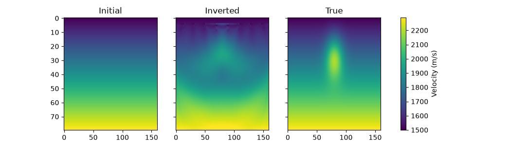
Over 200 iterations the data misfit falls by about two orders of magnitude and the model root-mean-square error falls from 66.5 to 58.8 m/s. The anomaly comes back in the right place with the right sign, but only part of its amplitude, and smeared vertically.
That is what the survey supports, not a defect of the inversion. Every source and receiver is at the surface, so the top of the model is crossed by many ray paths at many angles and the bottom by few at almost the same angle. Vertical smearing is the signature of narrow angular coverage; the corners beyond the outermost sources are barely updated at all because no ray reaches them. Before blaming the optimiser for a feature that will not resolve, ask whether anything in the recorded data constrains it. Widening the survey, recording for longer, adding lower frequencies, or putting receivers in a borehole all change what can be recovered – and none of them is a change to how the inversion is written.
Two other caveats worth stating plainly. The observed data here is generated with the same propagator the inversion uses, which makes this an “inverse crime”: there is no modelling error at all, so the inversion has an easier time of it than it would with recorded data. And the misfit is a plain mean-squared error on the raw traces, which is the most cycle-skipping-prone choice there is; see Graph Space Optimal Transport and FWI Recipes: Exotic Misfits, Deep Priors, and Uncertainty for alternatives.
Where to go next
Full-Waveform Inversion (FWI) – the same inversion on the Marmousi model, plus constrained velocities and a multi-scale frequency progression.
Reverse-Time Migration (RTM) – migration rather than inversion: one gradient with respect to a scattering potential.
FWI Recipes: Exotic Misfits, Deep Priors, and Uncertainty – optimal-transport and other misfits, deep priors, and uncertainty estimates, each a short addition to this loop.
FWI in other parameterisations – inverting for something other than velocity directly.
Troubleshooting – when an inversion diverges, stalls, or produces a model full of artefacts.