Full-Waveform Inversion (FWI)
Full-Waveform Inversion provides the potential to invert for a model that matches the whole recorded dataset, including refracted arrivals.
We continue with using the Marmousi model, but due to the computational cost of running many iterations of FWI, we will work on only a portion of it:
import torch
from scipy.ndimage import gaussian_filter
import matplotlib.pyplot as plt
import deepwave
from deepwave import scalar

device = torch.device('cuda' if torch.cuda.is_available()
                      else 'cpu')
ny = 2301
nx = 751
dx = 4.0
v_true = torch.from_file('marmousi_vp.bin',
                         size=ny*nx).reshape(ny, nx)

# Select portion of model for inversion
ny = 600
nx = 250
v_true = v_true[:ny, :nx]
We smooth the true model to create our initial guess of the wavespeed, which we will attempt to improve with inversion. We also load the data that we generated in the forward modelling example to serve as our target observed data:
v_init = (torch.tensor(1/gaussian_filter(1/v_true.numpy(), 40))
          .to(device))
v = v_init.clone()
v.requires_grad_()

n_shots = 115

n_sources_per_shot = 1
d_source = 20  # 20 * 4m = 80m
first_source = 10  # 10 * 4m = 40m
source_depth = 2  # 2 * 4m = 8m

n_receivers_per_shot = 384
d_receiver = 6  # 6 * 4m = 24m
first_receiver = 0  # 0 * 4m = 0m
receiver_depth = 2  # 2 * 4m = 8m

freq = 25
nt = 750
dt = 0.004
peak_time = 1.5 / freq

observed_data = (
    torch.from_file('marmousi_data.bin',
                    size=n_shots*n_receivers_per_shot*nt)
    .reshape(n_shots, n_receivers_per_shot, nt)
)
As our model is now smaller, we also need to extract only the portion of the observed data that covers this section of the model:
n_shots = 20
n_receivers_per_shot = 100
nt = 300
observed_data = (
    observed_data[:n_shots, :n_receivers_per_shot, :nt].to(device)
)
We set-up the sources and receivers as before:
# source_locations
source_locations = torch.zeros(n_shots, n_sources_per_shot, 2,
                               dtype=torch.long, device=device)
source_locations[..., 1] = source_depth
source_locations[:, 0, 0] = (torch.arange(n_shots) * d_source +
                             first_source)

# receiver_locations
receiver_locations = torch.zeros(n_shots, n_receivers_per_shot, 2,
                                 dtype=torch.long, device=device)
receiver_locations[..., 1] = receiver_depth
receiver_locations[:, :, 0] = (
    (torch.arange(n_receivers_per_shot) * d_receiver +
     first_receiver)
    .repeat(n_shots, 1)
)

# source_amplitudes
source_amplitudes = (
    (deepwave.wavelets.ricker(freq, nt, dt, peak_time))
    .repeat(n_shots, n_sources_per_shot, 1).to(device)
)
We are now ready to run the optimiser to perform iterative inversion of the wavespeed model. This will be achieved using code that is very similar to what would be used to train a typical neural network in PyTorch. The only notable differences are that we use a larger learning rate (1e9) to boost the gradient values to a range that will help us to make good progress with each iteration, and that we apply a clipping to the gradients (to the 98th percentile of their magnitude) to avoid making very large changes at a small number of points (such as around the sources):
# Setup optimiser to perform inversion
optimiser = torch.optim.SGD([v], lr=1e9, momentum=0.9)
loss_fn = torch.nn.MSELoss()

# Run optimisation/inversion
n_epochs = 250
v_true = v_true.to(device)

for epoch in range(n_epochs):
    optimiser.zero_grad()
    out = scalar(
        v, dx, dt,
        source_amplitudes=source_amplitudes,
        source_locations=source_locations,
        receiver_locations=receiver_locations,
        pml_freq=freq,
    )
    loss = loss_fn(out[-1], observed_data)
    loss.backward()
    torch.nn.utils.clip_grad_value_(
        v,
        torch.quantile(v.grad.detach().abs(), 0.98)
    )
    optimiser.step()
The result is an improvement in the accuracy of our estimate of the wavespeed model. Note that the sources do not cover a portion of the surface on the right, which is why the result is worse there.
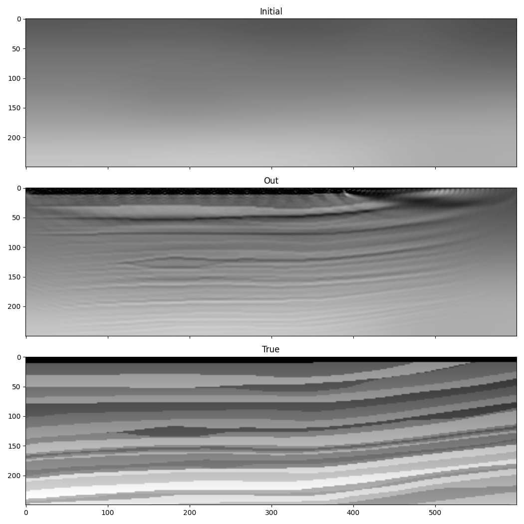
It looks like the low wavenumber information (the layer velocities) is missing from the lower part of the model, however. This is probably due to the cycle-skipping problem, a common issue in seismic inversion where the inversion gets stuck in a local minimum.
We thus encountered two problems. The first is the risk of velocity values in particular cells getting too large or small during the inversion and causing stability issues. This is caused by the gradient values being large near the sources and receivers, and the optimiser thus taking large steps there. We tried to address this by using gradient clipping. The second problem is cycle-skipping, where modelled arrivals being shifted by more than half a wavelength from their target counterparts can cause the inversion to get stuck in a local minimum. Let’s try to overcome these problems with some improvements to the code.
One approach to resolving the problem of extreme velocity values is to constrain the velocities to be within a desired range. Because PyTorch enables us to chain operators together and will automatically backpropagate through them to calculate gradients, we can use a function to generate our velocity model. This provides a convenient and robust way to constrain the range of velocities in our model. We can define our velocity model to be an object containing a tensor of the same size as our model. When we call the forward method of this object, it returns the output of applying the sigmoid operation to this stored tensor, resulting in a value between 0 and 1 for each cell, which is then scaled to our desired range. We can set the initial output of this to be our chosen initial velocity model using the logit operator, which is the inverse of sigmoid:
class Model(torch.nn.Module):
    def __init__(self, initial, min_vel, max_vel):
        super().__init__()
        self.min_vel = min_vel
        self.max_vel = max_vel
        self.model = torch.nn.Parameter(
            torch.logit((initial - min_vel) /
                        (max_vel - min_vel))
        )

    def forward(self):
        return (torch.sigmoid(self.model) *
                (self.max_vel - self.min_vel) +
                self.min_vel)


model = Model(v_init, 1000, 2500).to(device)
Now, when we create the optimiser, the tensor that we will ask it to optimise is the tensor inside this object. During backpropagation, the gradient of the loss function with respect to the velocity model will be further backpropagated to calculate the gradient with respect to this tensor. We therefore won’t be directly updating the velocity model, but will instead be updating this tensor that is used to generate the velocity model.
Next we will try to reduce the cycle-skipping problem. A common remedy is to initially use only the low frequencies in the data, and to gradually increase the maximum frequency that is used. Let’s use a simple implementation of this. We will progress from an initial cutoff frequency of 10 Hz in the early iterations, to 30 Hz in the final iterations. To keep this example simple we will apply the frequency filter to the output of wave propagation. In a more sophisticated implementation you would instead probably filter the source amplitudes, since a lower frequency source would allow you to use a larger grid cell spacing, reducing computational cost. To apply the frequency filter, we use a chain of second-order sections to implement a 6th order Butterworth filter with the biquad function from torchaudio and butter from scipy:
for cutoff_freq in [10, 15, 20, 25, 30]:
    sos = butter(6, cutoff_freq, fs=1/dt, output='sos')
    sos = [torch.tensor(sosi).to(observed_data.dtype).to(device)
           for sosi in sos]

    def filt(x):
        return biquad(biquad(biquad(x, *sos[0]), *sos[1]), *sos[2])
    observed_data_filt = filt(observed_data)
    optimiser = torch.optim.LBFGS(model.parameters(),
                                  line_search_fn='strong_wolfe')
    for epoch in range(n_epochs):
        def closure():
            optimiser.zero_grad()
            v = model()
            out = scalar(
                v, dx, dt,
                source_amplitudes=source_amplitudes,
                source_locations=source_locations,
                receiver_locations=receiver_locations,
                max_vel=2500,
                pml_freq=freq,
                time_pad_frac=0.2,
            )
            out_filt = filt(taper(out[-1]))
            loss = 1e6*loss_fn(out_filt, observed_data_filt)
            loss.backward()
            return loss

        optimiser.step(closure)
There are a few things to note here.
The first is that we switched to using the LBFGS optimiser. This allows me to demonstrate how to use it, since it is a bit different to other PyTorch optimisers. You have to put the loss and gradient calculation code inside a function, which is called closure in this example. This function is passed to the optimiser’s step method. You can use this approach with the other optimisers as well, so you might like to always write your code in this way as it then allows you to easily use any of the optimisers. Another change related to LBFGS is that a scaling (1e6 in this case) is applied to the loss. That is because the LBFGS optimiser stops when the values are smaller than a threshold. You can alternatively change LBFGS’s threshold value, but I find this easier. If you leave this scaling in place but switch to an optimiser that uses the gradient value to update the model, such as gradient descent, then you should decrease the optimiser’s learning rate by this scaling factor so that the size of the updates stays the same (since scaling the loss will scale the gradient, so the scaling will be cancelled out by the decrease in the learning rate). Note that we create a new optimiser each time we change the filter frequency. That is because it might confuse optimisers that consider the history of previous iterations, such as LBFGS, if we continued using the same optimiser even after such a big change.
The second is that there are a few other tweaks, such as specifying the maximum velocity for the wave propagator and the fraction of time padding to use (see the Usage section to learn what they do), and applying a taper function to the data (see the full code for its definition). This is partly done to show you that things like this are possible, and partly because they help to make the data cleaner and so might reduce artefacts.
From the results, especially the improvement in recovery of the low wavenumber features in the deeper part of the model, it seems like these changes successfully overcame some of the problems that we encountered with the very simple implementation.
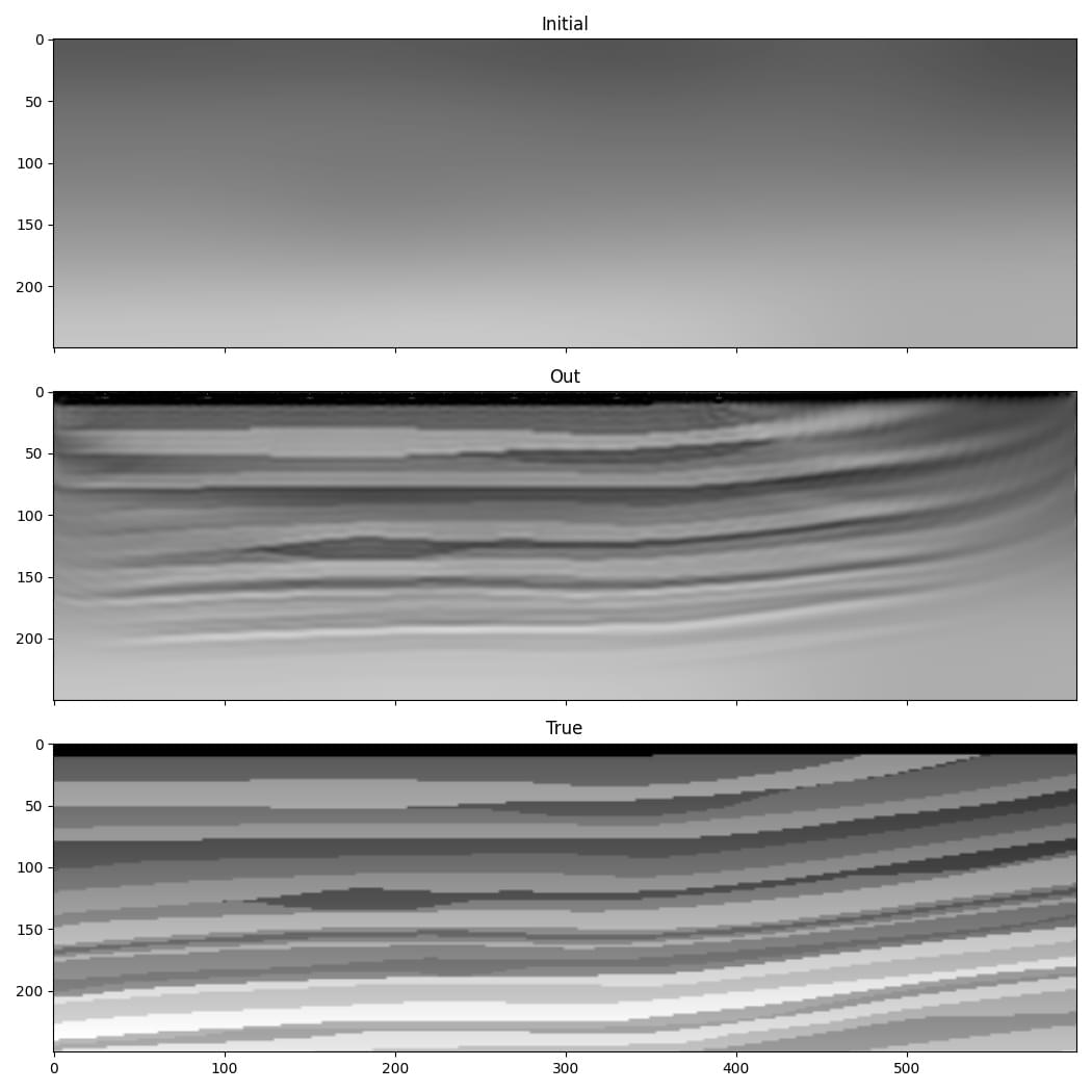
Even this is a simplified implementation of FWI, however, and it is unlikely to be sufficient for inverting real or even non-inverse crime data. It is not meant to be a recipe for how to perform FWI, but rather a demonstration of some of the things that are possible and a simple base on which you can build. Faster convergence and greater robustness in more realistic situations can be achieved with modifications such as a more sophisticated loss function. The advantage of basing Deepwave on PyTorch is that it means you can easily and quickly test ideas. As PyTorch will automatically backpropagate through any differentiable operations that you apply to the output of Deepwave, you only have to specify the forward action of such loss functions (or any other operations that you apply in the computational graph before or after Deepwave’s propagator) and can then let PyTorch automatically handle the backpropagation.