Forward modelling with Marmousi velocity model
In this example we will load the Marmousi 1 Vp (P-wave velocity) model, specify source and receiver locations, and then use Deepwave to perform forward modelling, propagating the sources through the model to generate synthetic receiver data.
First, we need to import the necessary packages:
import torch
import matplotlib.pyplot as plt
import deepwave
from deepwave import scalar
We then choose which device we wish to run on, specify the size of the model, and load it:
device = torch.device('cuda' if torch.cuda.is_available()
                      else 'cpu')
ny = 2301
nx = 751
dx = 4.0
v = torch.from_file('marmousi_vp.bin',
                    size=ny*nx).reshape(ny, nx).to(device)
At the time of writing, the Marmousi 1 velocity model can be downloaded from here.
Next we will specify where we wish to place the sources and receivers, and what the source wavelets should be. Deepwave can propagate batches of shots simultaneously to improve computational performance. These shots do not interact with each other, and the results are identical to propagating them individually. Shots propagated simultaneously are assumed to have the same number of sources and receivers. Their locations can be provided in Tensors with dimensions [shot, source, space] and [shot, receiver, space], respectively, and source amplitudes in a Tensor with dimensions [shot, source, time]. Many applications use only one source per shot, so the source dimension will often be of unit length, but Deepwave supports multiple sources per shot:
n_shots = 115

n_sources_per_shot = 1
d_source = 20  # 20 * 4m = 80m
first_source = 10  # 10 * 4m = 40m
source_depth = 2  # 2 * 4m = 8m

n_receivers_per_shot = 384
d_receiver = 6  # 6 * 4m = 24m
first_receiver = 0  # 0 * 4m = 0m
receiver_depth = 2  # 2 * 4m = 8m

freq = 25
nt = 750
dt = 0.004
peak_time = 1.5 / freq

# source_locations
source_locations = torch.zeros(n_shots, n_sources_per_shot, 2,
                               dtype=torch.long, device=device)
source_locations[..., 1] = source_depth
source_locations[:, 0, 0] = (torch.arange(n_shots) * d_source +
                             first_source)

# receiver_locations
receiver_locations = torch.zeros(n_shots, n_receivers_per_shot, 2,
                                 dtype=torch.long, device=device)
receiver_locations[..., 1] = receiver_depth
receiver_locations[:, :, 0] = (
    (torch.arange(n_receivers_per_shot) * d_receiver +
     first_receiver)
    .repeat(n_shots, 1)
)

# source_amplitudes
source_amplitudes = (
    deepwave.wavelets.ricker(freq, nt, dt, peak_time)
    .repeat(n_shots, n_sources_per_shot, 1)
    .to(device)
)
Both spatial dimensions are treated equally in Deepwave. In this example we chose to orient our velocity model so that dimension 0 is horizontal and dimension 1 is vertical, and specified our source and receiver locations in a way that is consistent with that, but we could have transposed the model and used dimension 0 as depth if we wished.
That’s all the setup that we need for forward modelling, so we are now ready to call Deepwave. As we would like to ensure that the results are as accurate as possible, we will specify that we wish to use 8th order accurate spatial finite differences:
out = scalar(v, dx, dt, source_amplitudes=source_amplitudes,
             source_locations=source_locations,
             receiver_locations=receiver_locations,
             accuracy=8,
             pml_freq=freq)
The pml_freq parameter is optional, but is recommended as it allows you to specify the dominant frequency to the PML, which helps to minimise edge reflections. You can see that the source and receiver Tensors that we provided were also optional. You can instead (or in addition) provide initial wavefields for Deepwave to propagate.
The number of time steps to propagate for (and thus the length of the output receiver data) is specified by the length of the source amplitude. If you are propagating without a source term, then you can instead specify it using the nt keyword parameter.
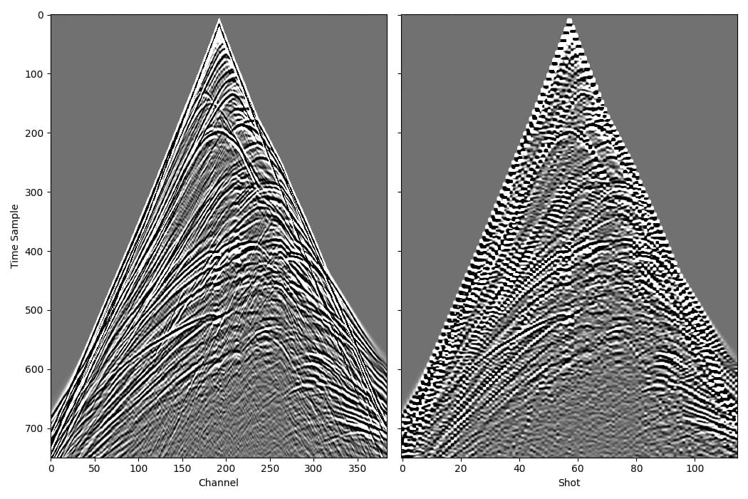
Finally, we will plot one common shot gather and one common receiver gather of the generated data, and then save the data to disk for use in later examples:
receiver_amplitudes = out[-1]
vmin, vmax = torch.quantile(receiver_amplitudes[0],
                            torch.tensor([0.05, 0.95]).to(device))
_, ax = plt.subplots(1, 2, figsize=(10.5, 7), sharey=True)
ax[0].imshow(receiver_amplitudes[57].cpu().T, aspect='auto',
             cmap='gray', vmin=vmin, vmax=vmax)
ax[1].imshow(receiver_amplitudes[:, 192].cpu().T, aspect='auto',
             cmap='gray', vmin=vmin, vmax=vmax)
ax[0].set_xlabel("Channel")
ax[0].set_ylabel("Time Sample")
ax[1].set_xlabel("Shot")
plt.tight_layout()

receiver_amplitudes.cpu().numpy().tofile('marmousi_data.bin')
We did not need to use them in this case, but if the output receiver amplitudes contain undesirable wraparound artefacts (where high amplitudes at the end of a trace cause artefacts at the beginning of the trace) then the Deepwave propagator options freq_taper_frac and time_pad_frac should be helpful. You can read more about them in the Usage section.