Elastic propagation and FWI
The regular scalar propagator has one model parameter (wavespeed). The scalar Born propagator has two (wavespeed and scattering potential). The elastic propagator has three. This makes it interesting to study as an inverse problem, because, in addition to the difficulties that already exist with scalar wave propagation inversion, there are problems caused by crosstalk between the model parameters. The ease of experimenting with different model parameterisations and loss functions makes Deepwave well suited to trying out new ideas to solve these problems. In this example we will just perform a simple forward propagation and inversion, though, to show you the basics.
One popular way to parameterise elastic propagation is with \(v_p\), \(v_s\), and \(\rho\) (the p and s wavespeeds and the density). Another uses \(\lambda\), \(\mu\), and buoyancy (the two Lamé parameters and the reciprocal of density). Deepwave internally uses the latter, and provides functions to convert between the two parameterisations. To demonstrate that you can parameterise the model any way that you like and use PyTorch’s end-to-end forward and backward propagation to update your own model parameters, in this example we will use \(v_p\), \(v_s\), and \(\rho\).
We begin by setting up the model (both background and true, the latter of which we will use to generate the “observed” data) and acquisition:
device = torch.device('cuda' if torch.cuda.is_available()
                      else 'cpu')
ny = 30
nx = 100
dx = 4.0

vp_background = torch.ones(ny, nx, device=device) * 1500
vs_background = torch.ones(ny, nx, device=device) * 1000
rho_background = torch.ones(ny, nx, device=device) * 2200

vp_true = vp_background.clone()
vp_true[10:20, 30:40] = 1600
vs_true = vs_background.clone()
vs_true[10:20, 45:55] = 1100
rho_true = rho_background.clone()
rho_true[10:20, 60:70] = 2300

n_shots = 8

n_sources_per_shot = 1
d_source = 12
first_source = 8
source_depth = 2

n_receivers_per_shot = nx-1
d_receiver = 1
first_receiver = 0
receiver_depth = 2

freq = 15
nt = 200
dt = 0.004
peak_time = 1.5 / freq

# source_locations
source_locations = torch.zeros(n_shots, n_sources_per_shot, 2,
                               dtype=torch.long, device=device)
source_locations[..., 0] = source_depth
source_locations[:, 0, 1] = (torch.arange(n_shots) * d_source +
                             first_source)

# receiver_locations
receiver_locations = torch.zeros(n_shots, n_receivers_per_shot, 2,
                                 dtype=torch.long, device=device)
receiver_locations[..., 0] = receiver_depth
receiver_locations[:, :, 1] = (
    (torch.arange(n_receivers_per_shot) * d_receiver +
     first_receiver)
    .repeat(n_shots, 1)
)

# source_amplitudes
source_amplitudes = (
    (deepwave.wavelets.ricker(freq, nt, dt, peak_time))
    .repeat(n_shots, n_sources_per_shot, 1).to(device)
)
This created a model where each of the three parameters is constant except for a box, which is in a different location for each parameter. We will use eight shots, with sources spread over the top surface, and receivers covering the top surface. Deepwave treats both spatial dimensions equally, so we could have transposed our model and defined our source and receiver locations with dimension 1 corresponding to depth instead of dimension 0. As a demonstration of this, this example uses the opposite convention of the earlier Marmousi examples. We are now ready to generate data using the true model:
observed_data = elastic(
    *deepwave.common.vpvsrho_to_lambmubuoyancy(vp_true, vs_true,
                                               rho_true),
    dx, dt,
    source_amplitudes_y=source_amplitudes,
    source_locations_y=source_locations,
    receiver_locations_y=receiver_locations,
    pml_freq=freq,
)[-2]
This is similar to how the scalar propagator is called, but with two differences.
The first is that we pass the three elastic model parameters. We are parameterising the model with \(v_p\), \(v_s\), and \(\rho\), but Deepwave wants us to provide them as \(\lambda\), \(\mu\), and buoyancy, so we convert them. Deepwave provides a function to do this, which we use here, but you can also create your own conversion function if you parameterise your model in some other way.
The elastic propagator can have sources and receivers oriented in each of the spatial dimensions. In this example we are only going to use sources and receivers that are oriented in the first (y) dimension. We could also provide receiver_locations_x if we wanted receivers that record particle velocity in the second dimension, for example.
Now let’s try starting from the background models (constant, without the boxes) and see if we can obtain something close to the true model when we invert with the true observed data:
vp = vp_background.clone().requires_grad_()
vs = vs_background.clone().requires_grad_()
rho = rho_background.clone().requires_grad_()
optimiser = torch.optim.LBFGS([vp, vs, rho])
loss_fn = torch.nn.MSELoss()

# Run optimisation/inversion
n_epochs = 20

for epoch in range(n_epochs):
    def closure():
        optimiser.zero_grad()
        out = elastic(
            *deepwave.common.vpvsrho_to_lambmubuoyancy(vp, vs, rho),
            dx, dt,
            source_amplitudes_y=source_amplitudes,
            source_locations_y=source_locations,
            receiver_locations_y=receiver_locations,
            pml_freq=freq,
        )[-2]
        loss = 1e20*loss_fn(out, observed_data)
        loss.backward()
        return loss

    optimiser.step(closure)
This just used a standard inversion with the LBFGS optimiser, but the result looks quite good.
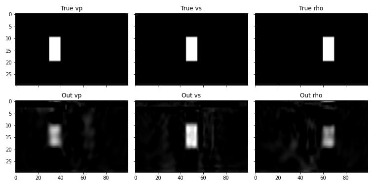
The gradients flowed end-to-end, back into the vp, vs, and rho parameters. You can see that there is a little bit of crosstalk between the parameters, though. Maybe you can come-up with a way of parameterising the model, or a different loss function, that does better?
Another interesting aspect of the elastic wave equation is that it can produce the phenomenon known as ground-roll. We can cause it by having a free surface on our model. Since Deepwave’s elastic propagator uses the improved vacuum method, we achieve this by setting the property models above the surface to zero (and we will also set the PML width to zero on that edge to avoid unnecessary computation, as no waves will reach the edge and so we do not need it to be absorbing):
vp[0] = 0
vs[0] = 0
rho[0] = 0
out = deepwave.elastic(
    *deepwave.common.vpvsrho_to_lambmubuoyancy(vp, vs,
                                               rho),
    grid_spacing=2, dt=0.004,
    source_amplitudes_y=(
        deepwave.wavelets.ricker(25, 50, 0.004, 0.06)
        .reshape(1, 1, -1)
    ),
    source_locations_y=torch.tensor([[[0, nx//2]]]),
    receiver_locations_y=x_r_y,
    receiver_locations_x=x_r_x,
    pml_width=[0, 20, 20, 20]
)
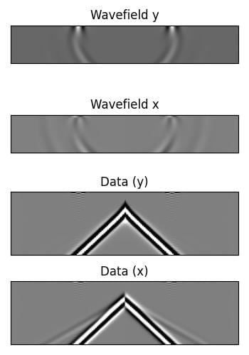
The same principle can be used to create a free surface of any shape. The following example demonstrates this by creating a model with a complex free surface (including voids) and recording the wavefield over time. The resulting animation shows the wave interacting with the complex free surface.

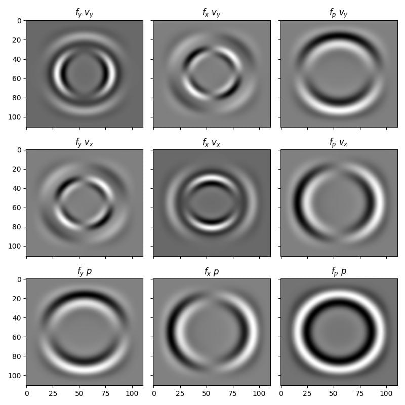
The elastic propagator supports three types of sources: body forces in the y and x dimensions (\(f_y\) and \(f_x\)), and pressure sources (\(f_p\)). We can compare these by looking at the resulting particle velocity in the y and x dimensions (\(v_y\) and \(v_x\)) and the pressure field (\(-\sigma_{yy}-\sigma_{xx}\), denoted \(p\)).