Born Modelling with the Elastic Wave Equation
Note
Stability: experimental – the label records that this propagator has never appeared in a release, so 0.1.0 is the first time real use meets its design. It is not a lesser promise: its interface is frozen exactly as the other ten propagators’ are, calling it emits no warning about its maturity, and every other Deepwave promise applies to it unchanged. See Stability policy.
This page describes deepwave.elastic_born(), Born (linearised) modelling for the isotropic elastic wave equation described in Elastic wave equation. It follows the same pattern as Born Modelling with the Scalar Wave Equation and Born Modelling with the Variable-Density Acoustic Wave Equation (read those pages first for the general idea of Born modelling in Deepwave), extended to elasticity’s Lamé-parameter/buoyancy model and full stress tensor.
Minimal example
deepwave.elastic_born() takes the same background model as deepwave.elastic() plus a scattering perturbation, here a localised change in the shear modulus dmu:
import torch
import deepwave

vp = 1500 * torch.ones(40, 40)
vs = 1000 * torch.ones(40, 40)
rho = 2200 * torch.ones(40, 40)
lamb, mu, buoyancy = deepwave.vpvsrho_to_lambmubuoyancy(vp, vs, rho)
dmu = torch.zeros(40, 40)
dmu[20, 20] = 0.3 * float(mu[20, 20])  # a small shear-modulus perturbation

out = deepwave.elastic_born(
    lamb, mu, buoyancy, grid_spacing=5, dt=0.001,
    dmu=dmu,
    source_amplitudes_y=deepwave.wavelets.ricker(25, 200, 0.001, 0.05).reshape(1, 1, -1),
    source_locations_y=torch.tensor([[[5, 20]]]),
    sc_receiver_locations_y=torch.tensor([[[35, 20]]]),
    pml_width=10,
    pml_freq=25,
)
out.sc_receiver_amplitudes_y  # the scattered (Born) vertical velocity, shape [1, 1, 200]
The recipe below expands this into a full example with a plot and a gradient.
Derivation
deepwave.elastic() solves the isotropic velocity-stress system built from the Lamé parameters \(\lambda\), \(\mu\) and buoyancy \(B = 1/\rho\). Perturbing the model, \(\lambda \to \lambda + \delta\lambda\), \(\mu \to \mu + \delta\mu\), \(B_i \to B_i + \delta B_i\), and splitting the fields into background and first-order scattered parts (\(\mathbf{v} = \bar{\mathbf{v}} + \delta\mathbf{v}\), \(\sigma = \bar\sigma + \delta\sigma\)) gives, at zeroth order, the ordinary background elastic system, and at first order a scattered system that is the same isotropic elastic operator as the background field, driven by virtual sources built entirely from the background field’s own strain-rate and stress-divergence terms times the scattering models (\(\delta\lambda\), \(\delta\mu\), \(\delta B_i\)). As with Born Modelling with the Variable-Density Acoustic Wave Equation, each scattering perturbation lives at the same staggered node as the model parameter it perturbs, so no interpolation of the scattering models themselves is required.
Because both fields obey the identical isotropic elastic operator, every result already established for deepwave.elastic() (staggered-grid layout, C-PML/M-PML absorbing boundaries, the IVM free-surface, per-field image parity) transfers unchanged to each field of the Born pair independently – this is a direct analogy, not a separate physics derivation. See Derivation: isotropic elastic Born (linearised) propagator for the full discrete derivation, including the coupled forward update, the scattered-only and full two-field adjoints, and the second-order (Hessian-vector product, forward-mode jvp) structure.
Implementation
Deepwave’s elastic Born propagator simultaneously simulates two coupled elastic fields on the same staggered grid and with the same boundary handling (including mpml_fraction and free-surface faces) as deepwave.elastic():
Background field \((\bar{\mathbf{v}}, \bar\sigma)\): propagates in the background model
lamb/mu/buoyancyexactly asdeepwave.elastic()would.Scattered field \((\delta\mathbf{v}, \delta\sigma)\): propagates in the same background model, driven by virtual sources built from the background field’s strain-rate and stress-divergence terms times the scattering models
dlamb/dmu/dbuoyancy.
For a small perturbation, the sum of the background and scattered outputs approximates the output of the regular deepwave.elastic() propagator run with the perturbed model lamb + dlamb/mu + dmu/buoyancy + dbuoyancy.
Inputs and outputs
The propagator takes the same background model as deepwave.elastic() (lamb, mu, buoyancy) plus the scattering perturbations dlamb, dmu, dbuoyancy, applied to that background model. Receiver data can be recorded from both fields independently: the sc_receiver_locations_* arguments record the scattered field (the elastic Born data, the basis of elastic LSRTM/FWI gradients), and the optional bg_receiver_locations_* arguments record the background field. See deepwave.elastic_born()’s signature below for the full set of per-component source/receiver arguments, doubled for the background/ scattered pair as in deepwave.elastic().
Alongside the receiver data, the output carries the final background and scattered wavefields plus one opaque auxiliary_state holding both fields’ absorbing-boundary memory variables. Passing the whole output back in as initial_state continues the propagation in a later call (see Usage).
Recipe: background and scattered fields
A small, self-contained recipe demonstrating deepwave.elastic_born(): build a background model from vp/vs/rho with deepwave.vpvsrho_to_lambmubuoyancy(), add a localised mu (shear modulus) scattering perturbation, and compare the background and scattered receiver gathers a single coupled call produces:
lamb, mu, buoyancy = deepwave.vpvsrho_to_lambmubuoyancy(vp, vs, rho)
dmu = (0.3 * mu * gaussian_blob).requires_grad_()

out = elastic_born(
    lamb, mu, buoyancy, dx, dt,
    dmu=dmu,
    source_amplitudes_y=source_amplitudes,
    source_locations_y=source_locations,
    sc_receiver_locations_y=sc_receiver_locations,
    bg_receiver_locations_y=sc_receiver_locations,
    pml_freq=freq,
    max_vel=max_vel,
)
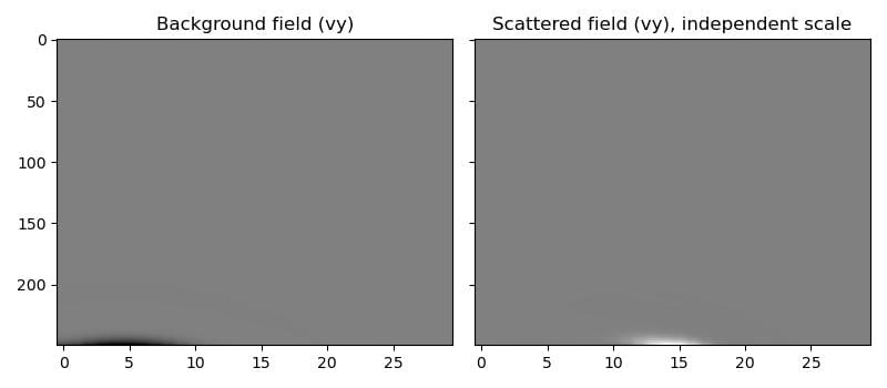
The scattered field is orders of magnitude weaker than the background field it rides on top of, for a scattering perturbation this small, but is clearly present as its own distinct arrival pattern (shown here on its own, independently normalised, colour scale) and is fully differentiable with respect to dmu – the basis of elastic LSRTM/FWI gradients (see LSRTM with the variable-density acoustic Born propagator for a full LSRTM inversion loop in the simpler variable-density acoustic case):
loss = out.sc_receiver_amplitudes_y.pow(2).sum()
loss.backward()
# dmu.grad is now populated and finite.
Specifying sources and receivers
The channel-keyed mapping form is the canonical way to specify a survey:
out = deepwave.elastic_born(
    ...,
    sources={"pressure_rate": (amplitudes, source_locations)},
    receivers={"p": receiver_locations},
    bg_receivers={"p": receiver_locations},
)
This propagator’s source channels are pressure_rate, z, y, x and its receiver channels are p, z, y, x (the z channel is absent in 2-D). "pressure_rate" names the quantity the scalar source injects; see Units and source conventions. "p" is still accepted there, with a deepwave.DeepwaveFutureWarning, and is removed in 0.4.0. It is unchanged as a receiver channel name. receivers= means the scattered receivers and bg_receivers= the background ones, matching the order of the returned tuple (background first, scattered second) and the sc_/bg_ flat spellings. The recorded data comes back as out.receivers[channel] and out.bg_receivers[channel].
The equivalent flat source_amplitudes_*/source_locations_*/ sc_receiver_locations_p keywords are equally permanent and produce bit-identical results; giving one channel in both forms raises. See Usage for the full vocabulary.